3-DOF Rocket Simulations#
RocketPy supports simplified 3-DOF (3 Degrees of Freedom) trajectory simulations, where the rocket is modeled as a point mass. This mode is useful for quick analyses, educational purposes, or when rotational dynamics are negligible.
Overview#
In a 3-DOF simulation, the rocket’s motion is described by three translational degrees of freedom (x, y, z positions), ignoring all rotational dynamics. This simplification:
Reduces computational complexity - Faster simulations for initial design studies
Focuses on trajectory - Ideal for apogee predictions and flight path analysis
Simplifies model setup - Requires fewer input parameters than full 6-DOF
When to Use 3-DOF Simulations#
3-DOF simulations are appropriate when:
You need quick trajectory estimates during preliminary design
Rotational stability is not a concern (e.g., highly stable rockets)
You’re performing educational demonstrations
You want to validate basic flight performance before detailed analysis
Warning
3-DOF simulations do not account for:
Rocket rotation and attitude dynamics
Stability margin and center of pressure effects
Aerodynamic moments and angular motion
Fin effectiveness and control surfaces
For complete flight analysis including stability, use standard 6-DOF simulations.
Setting Up a 3-DOF Simulation#
A 3-DOF simulation requires three main components:
rocketpy.PointMassMotor- Motor without rotational inertiarocketpy.PointMassRocket- Rocket without rotational propertiesrocketpy.Flightwithsimulation_mode="3 DOF"
Step 1: Define the Environment#
The environment setup is identical to standard simulations:
from rocketpy import Environment

env = Environment(
    latitude=32.990254,
    longitude=-106.974998,
    elevation=1400
)

env.set_atmospheric_model(type="standard_atmosphere")
Step 2: Create a PointMassMotor#
The rocketpy.PointMassMotor class represents a motor as a point mass,
without rotational inertia or grain geometry:
from rocketpy import PointMassMotor

# Using a thrust curve file
motor = PointMassMotor(
    thrust_source="../data/motors/cesaroni/Cesaroni_M1670.eng",
    dry_mass=1.815,
    propellant_initial_mass=2.5,
)
You can also define a constant thrust profile:
# Constant thrust of 250 N for 3 seconds
motor_constant = PointMassMotor(
    thrust_source=250,
    dry_mass=1.0,
    propellant_initial_mass=0.5,
    burn_time=3.0,
)
Or use a custom thrust function:
def custom_thrust(t):
    """Custom thrust profile: ramps up, plateaus, then ramps down"""
    if t < 0.5:
        return 500 * t / 0.5  # Ramp up
    elif t < 2.5:
        return 500  # Plateau
    elif t < 3.0:
        return 500 * (3.0 - t) / 0.5  # Ramp down
    else:
        return 0

motor_custom = PointMassMotor(
    thrust_source=custom_thrust,
    dry_mass=1.2,
    propellant_initial_mass=0.6,
    burn_time=3.0,
)
See also
For detailed information about rocketpy.PointMassMotor parameters,
see the rocketpy.PointMassMotor class documentation.
Step 3: Create a PointMassRocket#
The rocketpy.PointMassRocket class represents a rocket as a point mass:
from rocketpy import PointMassRocket

rocket = PointMassRocket(
    radius=0.0635,  # meters
    mass=5.0,  # kg (dry mass without motor)
    center_of_mass_without_motor=0.0,
    power_off_drag=0.5,  # Constant drag coefficient
    power_on_drag=0.5,
)

# Add the motor
rocket.add_motor(motor, position=0)
You can also specify drag as a function of Mach number:
# Drag coefficient vs Mach number
drag_curve = [
    [0.0, 0.50],
    [0.5, 0.48],
    [0.9, 0.52],
    [1.1, 0.65],
    [2.0, 0.55],
    [3.0, 0.50],
]

rocket_with_drag_curve = PointMassRocket(
    radius=0.0635,
    mass=5.0,
    center_of_mass_without_motor=0.0,
    power_off_drag=drag_curve,
    power_on_drag=drag_curve,
)
Note
Unlike the standard rocketpy.Rocket class, rocketpy.PointMassRocket
does not support:
Aerodynamic surfaces (fins, nose cones)
Inertia tensors
Center of pressure calculations
Stability margin analysis
Step 4: Run the Simulation#
Create a rocketpy.Flight object with simulation_mode="3 DOF":
from rocketpy import Flight

flight = Flight(
    rocket=rocket,
    environment=env,
    rail_length=5.2,
    inclination=85,  # degrees from horizontal
    heading=0,  # degrees (0 = North, 90 = East)
    simulation_mode="3 DOF",
    max_time=100,
    terminate_on_apogee=False,
)
Important
The simulation_mode="3 DOF" parameter is required to enable 3-DOF mode.
Without it, RocketPy will attempt a full 6-DOF simulation and may fail with
rocketpy.PointMassRocket.
Analyzing Results#
Once the simulation is complete, you can access trajectory data and generate plots.
Trajectory Information#
View key flight metrics:
flight.info()
Initial Conditions
Initial time: 0.000 s
Position - x: 0.00 m | y: 0.00 m | z: 1400.00 m
Velocity - Vx: 0.00 m/s | Vy: 0.00 m/s | Vz: 0.00 m/s
Attitude (quaternions) - e0: 0.999 | e1: -0.044 | e2: 0.000 | e3: 0.000
Euler Angles - Spin φ : 0.00° | Nutation θ: -5.00° | Precession ψ: 0.00°
Angular Velocity - ω1: 0.00 rad/s | ω2: 0.00 rad/s | ω3: 0.00 rad/s
Initial Stability Margin: 0.000 c
Surface Wind Conditions
Frontal Surface Wind Speed: 0.00 m/s
Lateral Surface Wind Speed: 0.00 m/s
Launch Rail
Launch Rail Length: 5.2 m
Launch Rail Inclination: 85.00°
Launch Rail Heading: 0.00°
Rail Departure State
Rail Departure Time: 0.304 s
Rail Departure Velocity: 44.941 m/s
Rail Departure Stability Margin: 0.000 c
Rail Departure Angle of Attack: 0.000°
Rail Departure Thrust-Weight Ratio: 20.681
Rail Departure Reynolds Number: 3.498e+05
Burn out State
Burn out time: 3.900 s
Altitude at burn out: 2695.401 m (ASL) | 1295.401 m (AGL)
Rocket speed at burn out: 476.469 m/s
Freestream velocity at burn out: 476.469 m/s
Mach Number at burn out: 1.447
Kinetic energy at burn out: 7.736e+05 J
Apogee State
Apogee Time: 24.246 s
Apogee Altitude: 5628.388 m (ASL) | 4228.388 m (AGL)
Apogee Freestream Speed: 20.490 m/s
Apogee X position: 0.000 m
Apogee Y position: 615.269 m
Apogee latitude: 32.9957865°
Apogee longitude: -106.9749980°
Parachute Events
No Parachute Events Were Triggered.
Impact Conditions
Time of impact: 46.665 s
X impact: 0.000 m
Y impact: 919.732 m
Altitude impact: 1399.999 m (ASL) | -0.001 m (AGL)
Latitude: 32.9985243°
Longitude: -106.9749980°
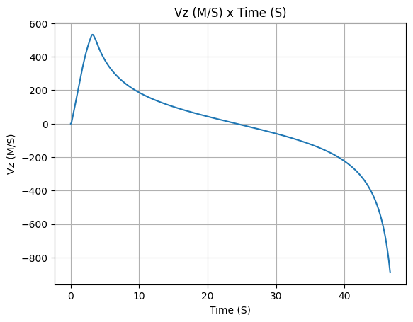
Vertical velocity at impact: -888.004 m/s
Number of parachutes triggered until impact: 0
Stability Margin
Initial Stability Margin: 0.000 c at 0.00 s
Out of Rail Stability Margin: 0.000 c at 0.30 s
Maximum Stability Margin: 0.000 c at 0.00 s
Minimum Stability Margin: 0.000 c at 0.00 s
Maximum Values
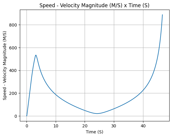
Maximum Speed: 888.817 m/s at 46.66 s
Maximum Mach Number: 2.657 Mach at 46.66 s
Maximum Reynolds Number: 6.921e+06 at 46.66 s
Maximum Dynamic Pressure: 4.221e+05 Pa at 46.66 s
Maximum Acceleration During Motor Burn: 227.845 m/s² at 0.15 s
Maximum Gs During Motor Burn: 23.234 g at 0.15 s
Maximum Acceleration After Motor Burn: 402.025 m/s² at 46.66 s
Maximum Gs After Motor Burn: 40.995 Gs at 46.66 s
Maximum Stability Margin: 0.000 c at 0.00 s
Numerical Integration Settings
Maximum Allowed Flight Time: 100.00 s
Maximum Allowed Time Step: inf s
Minimum Allowed Time Step: 0.00e+00 s
Relative Error Tolerance: 1e-06
Absolute Error Tolerance: [0.001, 0.001, 0.001, 0.001, 0.001, 0.001, 1e-06, 1e-06, 1e-06, 1e-06, 0.001, 0.001, 0.001]
Allow Event Overshoot: True
Terminate Simulation on Apogee: False
Number of Time Steps Used: 212
Number of Derivative Functions Evaluation: 402
Average Function Evaluations per Time Step: 1.896
This will display:
Apogee altitude and time
Maximum velocity
Flight time
Landing position
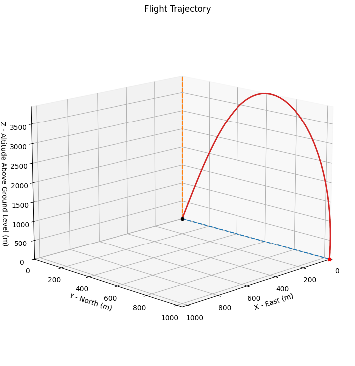
Plotting Trajectory#
Visualize the 3D flight path:
flight.plots.trajectory_3d()
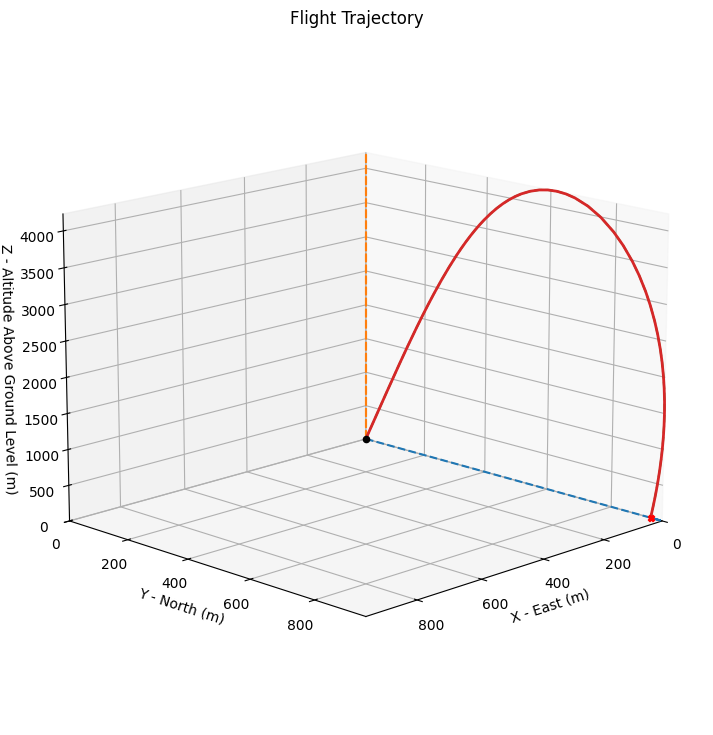
Note
In 3-DOF mode, the rocket maintains a fixed orientation (no pitch, yaw, or roll), so attitude plots are not meaningful.
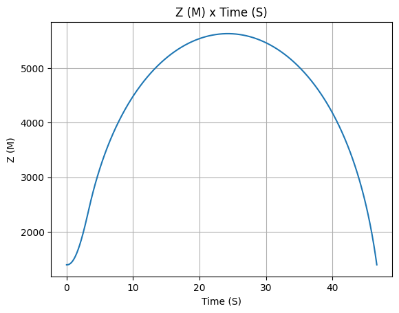
Available Plots#
The following plots are available for 3-DOF simulations:
# Altitude vs time
flight.z.plot()
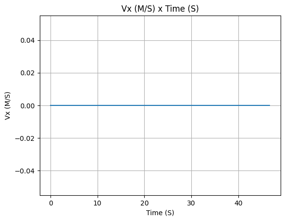
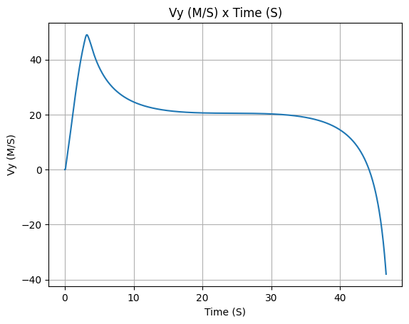
# Velocity components
flight.vx.plot()
flight.vy.plot()
flight.vz.plot()
# Total velocity
flight.speed.plot()
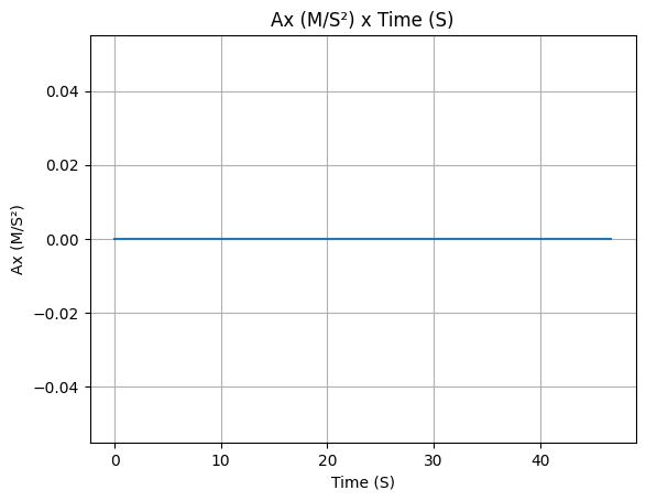
# Acceleration
flight.ax.plot()
Export Data#
Export trajectory data to CSV:
from rocketpy.simulation import FlightDataExporter

exporter = FlightDataExporter(flight)
exporter.export_data(
    "trajectory_3dof.csv",
    "x",
    "y",
    "z",
    "vx",
    "vy",
    "vz",
)
Complete Example#
Here’s a complete 3-DOF simulation from start to finish:
from rocketpy import Environment, PointMassMotor, PointMassRocket, Flight

# 1. Environment
env = Environment(
    latitude=39.3897,
    longitude=-8.2889,
    elevation=100
)
env.set_atmospheric_model(type="standard_atmosphere")

# 2. Motor
motor = PointMassMotor(
    thrust_source=1500,  # Constant 1500 N thrust
    dry_mass=2.0,
    propellant_initial_mass=3.0,
    burn_time=4.0,
)

# 3. Rocket
rocket = PointMassRocket(
    radius=0.0635,
    mass=8.0,
    center_of_mass_without_motor=0.0,
    power_off_drag=0.45,
    power_on_drag=0.45,
)
rocket.add_motor(motor, position=0)

# 4. Simulate
flight = Flight(
    rocket=rocket,
    environment=env,
    rail_length=5.2,
    inclination=85,
    heading=0,
    simulation_mode="3 DOF",
    max_time=120,
)

# 5. Results
print(f"Apogee: {flight.apogee:.2f} m")
print(f"Max velocity: {flight.max_speed:.2f} m/s")
print(f"Flight time: {flight.t_final:.2f} s")

flight.plots.trajectory_3d()
Apogee: 4045.23 m
Max velocity: 561.03 m/s
Flight time: 49.39 s
Weathercocking Model#
RocketPy’s 3-DOF simulation mode includes a weathercocking model that allows the rocket’s attitude to evolve during flight. This feature simulates how a statically stable rocket naturally aligns with the relative wind direction.
Understanding Weathercocking#
Weathercocking is the tendency of a rocket to align its body axis with the direction of the relative wind. In reality, this occurs due to aerodynamic restoring moments from fins and other stabilizing surfaces. The 3-DOF weathercocking model provides a simplified representation of this behavior without requiring full 6-DOF rotational dynamics.
The weathercocking coefficient (weathercock_coeff, often abbreviated
wc) represents the rate at which the rocket’s body axis aligns with
the relative wind. This simplified model does not consider aerodynamic
surfaces (for example, fins) or compute aerodynamic torques. In a
full 6-DOF model, weathercocking depends on quantities such as the
static margin and the normal-force coefficient, which produce restoring
moments that turn the rocket into the wind. A 3-DOF point-mass
simulation cannot compute those moments, so the model enforces
alignment of the body axis toward the freestream with a proportional
law.
Treat weathercock_coeff as a tuning parameter that approximates the
combined effect of static stability and restoring moments. It has no
direct physical units; designers typically select values by trial and
error and validate them later against full 6-DOF simulations.
Sources:
The weathercock_coeff Parameter#
The weathercocking behavior is controlled by the weathercock_coeff parameter
in the rocketpy.PointMassRocket class:
from rocketpy import Environment, PointMassMotor, PointMassRocket, Flight

env = Environment(
    latitude=32.990254,
    longitude=-106.974998,
    elevation=1400
)
env.set_atmospheric_model(type="standard_atmosphere")

motor = PointMassMotor(
    thrust_source=1500,
    dry_mass=1.5,
    propellant_initial_mass=2.5,
    burn_time=3.5,
)

rocket = PointMassRocket(
    radius=0.078,
    mass=15.0,
    center_of_mass_without_motor=0.0,
    power_off_drag=0.43,
    power_on_drag=0.43,
    weathercock_coeff=1.0,  # Example with weathercocking enabled
)
rocket.add_motor(motor, position=0)

# Flight uses the weathercocking configured on the point-mass rocket
flight = Flight(
    rocket=rocket,
    environment=env,
    rail_length=4.2,
    inclination=85,
    heading=45,
    simulation_mode="3 DOF",
)

print(f"Apogee: {flight.apogee - env.elevation:.2f} m")
Apogee: 2291.47 m
The weathercock_coeff parameter controls the rate at which the rocket
aligns with the relative wind:
weathercock_coeff=0: No weathercocking (original fixed-attitude behavior)weathercock_coeff=1.0: Moderate alignment rateweathercock_coeff>1.0: Faster alignment (more stable rocket)
Effect of Weathercocking Coefficient#
Higher values of weathercock_coeff result in faster alignment with the
relative wind. This affects the lateral motion and impact point:
Coefficient |
Alignment Speed |
Typical Use Case |
|---|---|---|
0 |
None (fixed attitude) |
Original 3-DOF behavior |
1.0 |
Moderate |
General purpose |
2.0-5.0 |
Fast |
Highly stable rockets |
>5.0 |
Very fast |
Rockets with large fins |
3-DOF vs 6-DOF Comparison Results#
The following example compares a 6-DOF simulation using the full Bella Lui rocket
with 3-DOF simulations using PointMassRocket and different weathercocking
coefficients. This demonstrates the trade-off between computational speed and
accuracy.
Note
The thrust curve files used in this example (e.g., AeroTech_K828FJ.eng)
are included in the RocketPy repository under the data/motors/ directory.
If you are running this code outside of the repository, you can download the
motor files from RocketPy’s data/motors folder on GitHub or use
your own thrust curve files.
Setup the simulations:
import numpy as np
import time
from rocketpy import Environment, Flight, Rocket, SolidMotor
from rocketpy.rocket.point_mass_rocket import PointMassRocket
from rocketpy.motors.point_mass_motor import PointMassMotor

# Environment
env = Environment(
    gravity=9.81,
    latitude=47.213476,
    longitude=9.003336,
    elevation=407,
)
env.set_atmospheric_model(type="standard_atmosphere")
env.max_expected_height = 2000

# Full 6-DOF Motor
motor_6dof = SolidMotor(
    thrust_source="../data/motors/aerotech/AeroTech_K828FJ.eng",
    burn_time=2.43,
    dry_mass=1,
    dry_inertia=(0, 0, 0),
    center_of_dry_mass_position=0,
    grains_center_of_mass_position=-1,
    grain_number=3,
    grain_separation=0.003,
    grain_density=782.4,
    grain_outer_radius=0.042799,
    grain_initial_inner_radius=0.033147,
    grain_initial_height=0.1524,
    nozzle_radius=0.04445,
    throat_radius=0.0214376,
    nozzle_position=-1.1356,
)

# Full 6-DOF Rocket
rocket_6dof = Rocket(
    radius=0.078,
    mass=17.227,
    inertia=(0.78267, 0.78267, 0.064244),
    power_off_drag=0.43,
    power_on_drag=0.43,
    center_of_mass_without_motor=0,
)
rocket_6dof.set_rail_buttons(0.1, -0.5)
rocket_6dof.add_motor(motor_6dof, -1.1356)
rocket_6dof.add_nose(length=0.242, kind="tangent", position=1.542)
rocket_6dof.add_trapezoidal_fins(3, span=0.200, root_chord=0.280, tip_chord=0.125, position=-0.75)

# Point Mass Motor for 3-DOF
motor_3dof = PointMassMotor(
    thrust_source="../data/motors/aerotech/AeroTech_K828FJ.eng",
    dry_mass=1.0,
    propellant_initial_mass=1.373,
)

# Point Mass Rocket for 3-DOF
rocket_3dof = PointMassRocket(
    radius=0.078,
    mass=17.227,
    center_of_mass_without_motor=0,
    power_off_drag=0.43,
    power_on_drag=0.43,
    weathercock_coeff=0.0,
)
rocket_3dof.add_motor(motor_3dof, -1.1356)
Run simulations and compare results:
# 6-DOF Flight
start = time.time()
flight_6dof = Flight(
    rocket=rocket_6dof,
    environment=env,
    rail_length=4.2,
    inclination=89,
    heading=45,
    terminate_on_apogee=True,
)
time_6dof = time.time() - start

# 3-DOF with no weathercocking
start = time.time()
rocket_3dof.weathercock_coeff = 0.0
flight_3dof_0 = Flight(
    rocket=rocket_3dof,
    environment=env,
    rail_length=4.2,
    inclination=89,
    heading=45,
    terminate_on_apogee=True,
    simulation_mode="3 DOF",
)
time_3dof_0 = time.time() - start

# 3-DOF with default weathercocking
start = time.time()
rocket_3dof.weathercock_coeff = 1.0
flight_3dof_1 = Flight(
    rocket=rocket_3dof,
    environment=env,
    rail_length=4.2,
    inclination=89,
    heading=45,
    terminate_on_apogee=True,
    simulation_mode="3 DOF",
)
time_3dof_1 = time.time() - start

# 3-DOF with high weathercocking
start = time.time()
rocket_3dof.weathercock_coeff = 5.0
flight_3dof_5 = Flight(
    rocket=rocket_3dof,
    environment=env,
    rail_length=4.2,
    inclination=89,
    heading=45,
    terminate_on_apogee=True,
    simulation_mode="3 DOF",
)
time_3dof_5 = time.time() - start

# Print comparison table
print("=" * 80)
print("SIMULATION RESULTS COMPARISON")
print("=" * 80)
print("\n{:<30} {:>12} {:>12} {:>12} {:>12}".format(
    "Parameter", "6-DOF", "3DOF(wc=0)", "3DOF(wc=1)", "3DOF(wc=5)"
))
print("-" * 80)
print("{:<30} {:>12.2f} {:>12.2f} {:>12.2f} {:>12.2f}".format(
    "Apogee (m AGL)",
    flight_6dof.apogee - env.elevation,
    flight_3dof_0.apogee - env.elevation,
    flight_3dof_1.apogee - env.elevation,
    flight_3dof_5.apogee - env.elevation,
))
print("{:<30} {:>12.2f} {:>12.2f} {:>12.2f} {:>12.2f}".format(
    "Apogee Time (s)",
    flight_6dof.apogee_time,
    flight_3dof_0.apogee_time,
    flight_3dof_1.apogee_time,
    flight_3dof_5.apogee_time,
))
print("{:<30} {:>12.2f} {:>12.2f} {:>12.2f} {:>12.2f}".format(
    "Max Speed (m/s)",
    flight_6dof.max_speed,
    flight_3dof_0.max_speed,
    flight_3dof_1.max_speed,
    flight_3dof_5.max_speed,
))
print("{:<30} {:>12.3f} {:>12.3f} {:>12.3f} {:>12.3f}".format(
    "Runtime (s)",
    time_6dof,
    time_3dof_0,
    time_3dof_1,
    time_3dof_5,
))
print("-" * 80)
print("Speedup vs 6-DOF:             {:>12} {:>12.1f}x {:>12.1f}x {:>12.1f}x".format(
    "-",
    time_6dof / time_3dof_0 if time_3dof_0 > 0 else 0,
    time_6dof / time_3dof_1 if time_3dof_1 > 0 else 0,
    time_6dof / time_3dof_5 if time_3dof_5 > 0 else 0,
))
================================================================================
SIMULATION RESULTS COMPARISON
================================================================================

Parameter                             6-DOF   3DOF(wc=0)   3DOF(wc=1)   3DOF(wc=5)
--------------------------------------------------------------------------------
Apogee (m AGL)                       461.62       448.65       448.31       448.32
Apogee Time (s)                       10.62        10.50        10.49        10.49
Max Speed (m/s)                       86.29        84.79        84.75        84.76
Runtime (s)                           0.270        0.024        0.038        0.042
--------------------------------------------------------------------------------
Speedup vs 6-DOF:                        -         11.1x          7.1x          6.5x
3D Trajectory Comparison:
import matplotlib.pyplot as plt
from mpl_toolkits.mplot3d import Axes3D

fig = plt.figure(figsize=(12, 8))
ax = fig.add_subplot(111, projection="3d")

# Plot all trajectories
ax.plot(flight_6dof.x[:, 1], flight_6dof.y[:, 1], flight_6dof.z[:, 1] - env.elevation,
        "b-", linewidth=2, label="6-DOF")
ax.plot(flight_3dof_0.x[:, 1], flight_3dof_0.y[:, 1], flight_3dof_0.z[:, 1] - env.elevation,
        "r--", linewidth=2, label="3-DOF (wc=0)")
ax.plot(flight_3dof_1.x[:, 1], flight_3dof_1.y[:, 1], flight_3dof_1.z[:, 1] - env.elevation,
        "g--", linewidth=2, label="3-DOF (wc=1)")
ax.plot(flight_3dof_5.x[:, 1], flight_3dof_5.y[:, 1], flight_3dof_5.z[:, 1] - env.elevation,
        "m--", linewidth=2, label="3-DOF (wc=5)")

ax.set_xlabel("X (m)")
ax.set_ylabel("Y (m)")
ax.set_zlabel("Altitude AGL (m)")
ax.set_title("3-DOF vs 6-DOF Trajectory Comparison with Weathercocking")
ax.legend()
plt.tight_layout()
plt.show()

The results show that:
3-DOF is 5-7x faster than 6-DOF simulations
Apogee prediction is within 1-3% of 6-DOF
Weathercocking improves trajectory accuracy by aligning the rocket with relative wind
Higher weathercock_coeff values result in trajectories closer to 6-DOF
Comparison: 3-DOF vs 6-DOF#
Understanding the differences between simulation modes:
Feature |
3-DOF |
6-DOF |
|---|---|---|
Computational Speed |
5-7x faster |
Slower (more accurate) |
Rocket Orientation |
Weathercocking model |
Full attitude dynamics |
Stability Analysis |
❌ Not available |
✅ Full stability margin |
Aerodynamic Surfaces |
❌ Not modeled |
✅ Fins, nose, tail |
Center of Pressure |
❌ Not computed |
✅ Computed |
Moments of Inertia |
❌ Not needed |
✅ Required |
Use Cases |
Quick estimates, Monte Carlo |
Detailed design, stability |
Trajectory Accuracy |
Good (~1.5% error) |
Highly accurate |
Best Practices#
Validate with 6-DOF: After getting initial results with 3-DOF, validate critical designs with full 6-DOF simulations.
Check Drag Coefficient: Ensure your drag coefficient is realistic for your rocket’s geometry. Use wind tunnel data or CFD if available.
Use Realistic Launch Conditions: Even in 3-DOF mode, wind conditions and rail length affect trajectory.
Document Assumptions: Clearly document that your analysis uses 3-DOF and its limitations.
Limitations and Warnings#
Danger
Critical Limitations:
No stability checking - The simulation cannot detect unstable rockets
No attitude control - Air brakes and thrust vectoring are not supported
Simplified weathercocking - Uses proportional alignment model, not full dynamics
Warning
3-DOF simulations should not be used for:
Final design verification
Stability margin analysis
Control system design
Fin sizing and optimization
Safety-critical trajectory predictions
See Also#
First Simulation - Standard 6-DOF simulation tutorial
Rocket Class Usage - Full rocket modeling capabilities
Flight Class Usage - Complete flight simulation options
Further Reading#
For more information about point mass trajectory simulations: