First Simulation with RocketPy#
Here we will show how to set up a complete simulation with RocketPy.
See also
You can find all the code used in this page in the notebooks folder of the RocketPy repository. You can also run the code in Google Colab:
RocketPy is structured into four main classes, each one with its own purpose:
Environment- Keeps data related to weather.Motor- Subdivided into SolidMotor, HybridMotor and LiquidMotor. Keeps data related to rocket motors.Rocket- Keeps data related to a rocket.Flight- Runs the simulation and keeps the results.
By using these four classes, we can create a complete simulation of a rocket flight.
The following image shows how the four main classes interact with each other to generate a rocket flight simulation:

Setting Up a Simulation#
A basic simulation with RocketPy is composed of the following steps:
Defining a
Environment,MotorandRocketobject.Running the simulation by defining a
Flightobject.Plotting/Analyzing the results.
Tip
It is recommended that RocketPy is ran in a Jupyter Notebook. This way, the results can be easily plotted and analyzed.
The first step to set up a simulation, we need to first import the classes we will use from RocketPy:
from rocketpy import Environment, SolidMotor, Rocket, Flight
Note
Here we will use a SolidMotor as an example, but the same steps can be applied to Hybrid and Liquid motors.
Defining a Environment#
The Environment class is used to store data related to the weather and the
wind conditions of the launch site. The weather conditions are imported from
weather organizations such as NOAA and ECMWF.
To define a Environment object, we need to first specify some information regarding the launch site:
env = Environment(latitude=32.990254, longitude=-106.974998, elevation=1400)
Next, we need to specify the atmospheric model to be used. In this example, we will get GFS forecasts data from tomorrow.
First we must set the date of the simulation. The date must be given in a tuple
with the following format: (year, month, day, hour).
The hour is given in UTC time. Here we use the datetime library to get the date
of tomorrow:
import datetime

tomorrow = datetime.date.today() + datetime.timedelta(days=1)

env.set_date(
    (tomorrow.year, tomorrow.month, tomorrow.day, 12)
)  # Hour given in UTC time
env.set_atmospheric_model(type="Forecast", file="GFS")
See also
To learn more about the different types of atmospheric models and a better description of the initialization parameters, see Environment Usage.
We can see what the weather will look like by calling the info method:
env.info()
Gravity Details

Acceleration of Gravity at Lauch Site: 9.79111266229703 m/s²


Launch Site Details

Launch Date: 2023-09-24 12:00:00 UTC
Launch Site Latitude: 32.99025°
Launch Site Longitude: -106.97500°
Reference Datum: SIRGAS2000
Launch Site UTM coordinates: 315468.64 W    3651938.65 N
Launch Site UTM zone: 13S
Launch Site Surface Elevation: 1471.5 m


Atmospheric Model Details

Atmospheric Model Type: Forecast
Forecast Maximum Height: 79.220 km
Forecast Time Period: From  2023-09-23 00:00:00  to  2023-10-09 00:00:00  UTC
Forecast Hour Interval: 3  hrs
Forecast Latitude Range: From  -90.0 ° To  90.0 °
Forecast Longitude Range: From  0.0 ° To  359.75 °


Surface Atmospheric Conditions

Surface Wind Speed: 4.32 m/s
Surface Wind Direction: 4.77°
Surface Wind Heading: 184.77°
Surface Pressure: 852.97 hPa
Surface Temperature: 295.02 K
Surface Air Density: 1.007 kg/m³
Surface Speed of Sound: 344.33 m/s


Atmospheric Model Plots

Defining a Motor#
RocketPy can simulate Solid, Hybrid and Liquid motors. Each type of
motor has its own class: rocketpy.SolidMotor,
rocketpy.HybridMotor and rocketpy.LiquidMotor.
In this example, we will use a SolidMotor. To define a SolidMotor, we need
to specify several parameters:
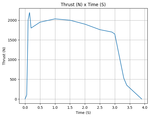
Pro75M1670 = SolidMotor(
    thrust_source="../data/motors/Cesaroni_M1670.eng",
    dry_mass=1.815,
    dry_inertia=(0.125, 0.125, 0.002),
    nozzle_radius=33 / 1000,
    grain_number=5,
    grain_density=1815,
    grain_outer_radius=33 / 1000,
    grain_initial_inner_radius=15 / 1000,
    grain_initial_height=120 / 1000,
    grain_separation=5 / 1000,
    grains_center_of_mass_position=0.397,
    center_of_dry_mass_position=0.317,
    nozzle_position=0,
    burn_time=3.9,
    throat_radius=11 / 1000,
    coordinate_system_orientation="nozzle_to_combustion_chamber",
)
Pro75M1670.info()
Nozzle Details
Nozzle Radius: 0.033 m
Nozzle Throat Radius: 0.011 m

Grain Details
Number of Grains: 5
Grain Spacing: 0.005 m
Grain Density: 1815 kg/m3
Grain Outer Radius: 0.033 m
Grain Inner Radius: 0.015 m
Grain Height: 0.12 m
Grain Volume: 0.000 m3
Grain Mass: 0.591 kg

Motor Details
Total Burning Time: 3.9 s
Total Propellant Mass: 2.956 kg
Average Propellant Exhaust Velocity: 2038.745 m/s
Average Thrust: 1545.218 N
Maximum Thrust: 2200.0 N at 0.15 s after ignition.
Total Impulse: 6026.350 Ns
Defining a Rocket#
To create a complete Rocket object, we need to complete some steps:
Define the rocket itself by passing in the rocket’s dry mass, inertia, drag coefficient and radius;
Add a motor;
Add, if desired, aerodynamic surfaces;
Add, if desired, parachutes;
Set, if desired, rail guides;
See results.
See also
To learn more about each step, see Rocket Class Usage
To create a Rocket object, we need to specify some parameters.
calisto = Rocket(
    radius=127 / 2000,
    mass=14.426,
    inertia=(6.321, 6.321, 0.034),
    power_off_drag="../data/calisto/powerOffDragCurve.csv",
    power_on_drag="../data/calisto/powerOnDragCurve.csv",
    center_of_mass_without_motor=0,
    coordinate_system_orientation="tail_to_nose",
)
Next, we need to add a Motor object to the Rocket object:
calisto.add_motor(Pro75M1670, position=-1.255)
We can also add rail guides to the rocket. These are not necessary for a simulation, but they are useful for a more realistic out of rail velocity and stability calculation.
rail_buttons = calisto.set_rail_buttons(
    upper_button_position=0.0818,
    lower_button_position=-0.6182,
    angular_position=45,
)
Then, we can add any number of Aerodynamic Components to the Rocket object.
Here we create a rocket with a nose cone, four fins and a tail:
nose_cone = calisto.add_nose(
    length=0.55829, kind="von karman", position=1.278
)

fin_set = calisto.add_trapezoidal_fins(
    n=4,
    root_chord=0.120,
    tip_chord=0.060,
    span=0.110,
    position=-1.04956,
    cant_angle=0.5,
    airfoil=("../data/calisto/NACA0012-radians.csv","radians"),
)

tail = calisto.add_tail(
    top_radius=0.0635, bottom_radius=0.0435, length=0.060, position=-1.194656
)
Due to the chosen bluffness ratio, the nose cone length was reduced to 0.558 m.
Finally, we can add any number of Parachutes to the Rocket object.
main = calisto.add_parachute(
    name="main",
    cd_s=10.0,
    trigger=800,      # ejection altitude in meters
    sampling_rate=105,
    lag=1.5,
    noise=(0, 8.3, 0.5),
)

drogue = calisto.add_parachute(
    name="drogue",
    cd_s=1.0,
    trigger="apogee",  # ejection at apogee
    sampling_rate=105,
    lag=1.5,
    noise=(0, 8.3, 0.5),
)
We can then see if the rocket is stable by plotting the static margin:
calisto.plots.static_margin()
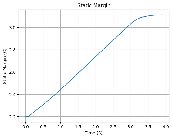
Danger
Always check the static margin of your rocket.
If it is negative, your rocket is unstable and the simulation will most likely fail.
If it is unreasonably high, your rocket is super stable and the simulation will most likely fail.
Running the Simulation#
To simulate a flight, we need to create a Flight object.
This object will run the simulation and store the results.
To do this, we need to specify the environment in which the rocket will fly and the rocket itself. We must also specify the length of the launch rail, the inclination of the launch rail and the heading of the launch rail.
test_flight = Flight(
    rocket=calisto, environment=env, rail_length=5.2, inclination=85, heading=0
    )
All simulation information will be saved in the test_flight.
There are several methods to access the results. For example, we can plot the speed of the rocket until the first parachute is deployed:
test_flight.speed.plot(0, test_flight.apogee_time)

Or get the array of the speed of the entire flight, in the form
of [[time, speed], ...]:
test_flight.speed.source
array([[0.00000000e+00, 0.00000000e+00],
       [1.40957093e-03, 0.00000000e+00],
       [2.81914187e-03, 0.00000000e+00],
       ...,
       [3.07766558e+02, 6.84800900e+00],
       [3.08384190e+02, 6.84460023e+00],
       [3.08411959e+02, 6.84444582e+00]])
See also
The Flight object has several attributes containing every result of the
simulation. To see all the attributes of the Flight object, see
rocketpy.Flight.
To see a very large summary of the results, we can call the all_info method:
test_flight.all_info()
Initial Conditions

Position - x: 0.00 m | y: 0.00 m | z: 1471.47 m
Velocity - Vx: 0.00 m/s | Vy: 0.00 m/s | Vz: 0.00 m/s
Attitude - e0: 0.999 | e1: -0.044 | e2: -0.000 | e3: 0.000
Euler Angles - Spin φ : 0.00° | Nutation θ: -5.00° | Precession ψ: 0.00°
Angular Velocity - ω1: 0.00 rad/s | ω2: 0.00 rad/s| ω3: 0.00 rad/s


Surface Wind Conditions

Frontal Surface Wind Speed: -4.31 m/s
Lateral Surface Wind Speed: 0.36 m/s


Launch Rail

Launch Rail Length: 5.2  m
Launch Rail Inclination: 85.00°
Launch Rail Heading: 0.00°


Rail Departure State

Rail Departure Time: 0.372 s
Rail Departure Velocity: 26.564 m/s
Rail Departure Static Margin: 2.273 c
Rail Departure Angle of Attack: 9.096°
Rail Departure Thrust-Weight Ratio: 10.165
Rail Departure Reynolds Number: 1.914e+05


Burn out State

Burn out time: 3.900 s
Altitude at burn out: 653.742 m (AGL)
Rocket velocity at burn out: 281.171 m/s
Freestream velocity at burn out: 281.637 m/s
Mach Number at burn out: 0.822
Kinetic energy at burn out: 6.420e+05 J


Apogee State

Apogee Altitude: 4790.001 m (ASL) | 3318.535 m (AGL)
Apogee Time: 25.973 s
Apogee Freestream Speed: 31.837 m/s


Parachute Events

Drogue Ejection Triggered at: 25.981 s
Drogue Parachute Inflated at: 27.481 s
Drogue Parachute Inflated with Freestream Speed of: 34.843 m/s
Drogue Parachute Inflated at Height of: 3307.538 m (AGL)
Main Ejection Triggered at: 164.200 s
Main Parachute Inflated at: 165.700 s
Main Parachute Inflated with Freestream Speed of: 17.442 m/s
Main Parachute Inflated at Height of: 775.559 m (AGL)


Impact Conditions

X Impact: 1818.943 m
Y Impact: 846.004 m
Time of Impact: 308.412 s
Velocity at Impact: -5.299 m/s


Maximum Values

Maximum Speed: 286.923 m/s at 3.39 s
Maximum Mach Number: 0.837 Mach at 3.39 s
Maximum Reynolds Number: 1.925e+06 at 3.32 s
Maximum Dynamic Pressure: 3.948e+04 Pa at 3.35 s
Maximum Acceleration During Motor Burn: 105.251 m/s² at 0.15 s
Maximum Gs During Motor Burn: 10.733 g at 0.15 s
Maximum Acceleration After Motor Burn: 10.161 m/s² at 20.39 s
Maximum Gs After Motor Burn: 1.036 g at 20.39 s
Maximum Upper Rail Button Normal Force: 2.857 N
Maximum Upper Rail Button Shear Force: 2.413 N
Maximum Lower Rail Button Normal Force: 1.302 N
Maximum Lower Rail Button Shear Force: 1.101 N


Numerical Integration Settings

Maximum Allowed Flight Time: 600.000000 s
Maximum Allowed Time Step: inf s
Minimum Allowed Time Step: 0.000000e+00 s
Relative Error Tolerance:  1e-06
Absolute Error Tolerance:  [0.001, 0.001, 0.001, 0.001, 0.001, 0.001, 1e-06, 1e-06, 1e-06, 1e-06, 0.001, 0.001, 0.001]
Allow Event Overshoot:  True
Terminate Simulation on Apogee:  False
Number of Time Steps Used:  1362
Number of Derivative Functions Evaluation:  2777
Average Function Evaluations per Time Step: 2.038913


Trajectory 3d Plot

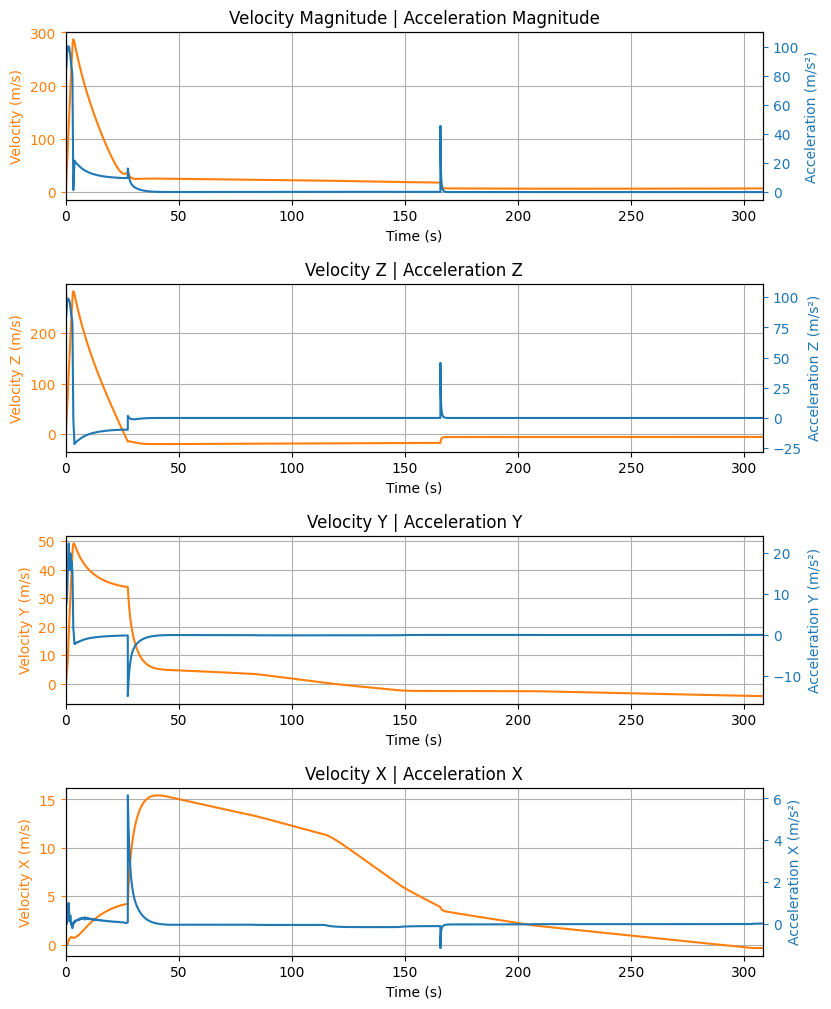
Trajectory Kinematic Plots
Angular Position Plots

Path, Attitude and Lateral Attitude Angle plots

Trajectory Angular Velocity and Acceleration Plots

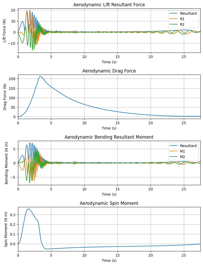
Aerodynamic Forces Plots
Rail Buttons Forces Plots

Trajectory Energy Plots
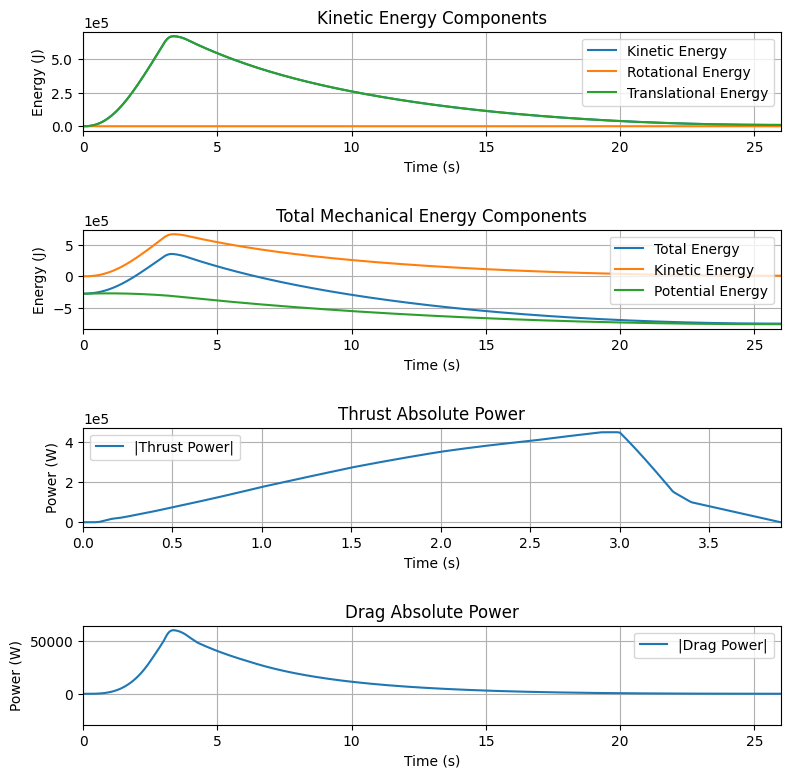
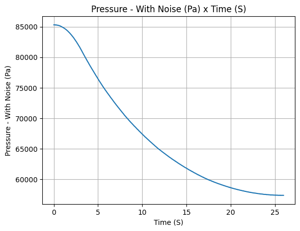
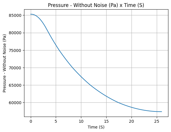
Trajectory Fluid Mechanics Plots

Trajectory Stability and Control Plots

Rocket and Parachute Pressure Plots

Parachute: main


Parachute: drogue

.kml to visualize it in Google Earth:test_flight.export_kml(
file_name="trajectory.kml",
extrude=True,
altitude_mode="relative_to_ground",
)
Further Analysis#
With the results of the simulation in hand, we can perform a lot of different analysis. Here we will show some examples, but much more can be done!
See also
RocketPy can be used to perform a Monte Carlo Dispersion Analysis. See Monte Carlo Simulations for more information.
Apogee as a Function of Mass#
This one is a classic! We always need to know how much our rocket’s apogee will change when our payload gets heavier.
from rocketpy.utilities import apogee_by_mass

apogee_by_mass(
    flight=test_flight, min_mass=5, max_mass=20, points=10, plot=True
    )

'Function from R1 to R1 : (Rocket Dry Mass (kg)) → (Estimated Apogee AGL (m))'
Out of Rail Speed as a Function of Mass#
Lets make a really important plot. Out of rail speed is the speed our rocket has when it is leaving the launch rail. This is crucial to make sure it can fly safely after leaving the rail.
A common rule of thumb is that our rocket’s out of rail speed should be 4 times the wind speed so that it does not stall and become unstable.
from rocketpy.utilities import liftoff_speed_by_mass

liftoff_speed_by_mass(
    flight=test_flight, min_mass=5, max_mass=20, points=10, plot=True
    )

'Function from R1 to R1 : (Rocket Dry Mass (kg)) → (Liftoff Speed (m/s))'
Dynamic Stability Analysis#
Ever wondered how static stability translates into dynamic stability? Different static margins result in different dynamic behavior, which also depends on the rocket’s rotational inertial.
Let’s make use of RocketPy’s helper class called Function to explore how the dynamic stability of Calisto varies if we change the fins span by a certain factor.
# Helper class
from rocketpy import Function
import copy

# Prepare a copy of the rocket
calisto2 = copy.deepcopy(calisto)

# Prepare Environment Class
custom_env = Environment()
custom_env.set_atmospheric_model(type="custom_atmosphere", wind_v=-5)

# Simulate Different Static Margins by Varying Fin Position
simulation_results = []

for factor in [-0.5, -0.2, 0.1, 0.4, 0.7]:
    # Modify rocket fin set by removing previous one and adding new one
    calisto2.aerodynamic_surfaces.pop(-1)

    fin_set = calisto2.add_trapezoidal_fins(
        n=4,
        root_chord=0.120,
        tip_chord=0.040,
        span=0.100,
        position=-1.04956 * factor,
    )
    # Simulate
    test_flight = Flight(
        rocket=calisto2,
        environment=custom_env,
        rail_length=5.2,
        inclination=90,
        heading=0,
        max_time_step=0.01,
        max_time=5,
        terminate_on_apogee=True,
        verbose=False,
    )
    # Store Results
    static_margin_at_ignition = calisto2.static_margin(0)
    static_margin_at_out_of_rail = calisto2.static_margin(test_flight.out_of_rail_time)
    static_margin_at_steady_state = calisto2.static_margin(test_flight.t_final)
    simulation_results += [
        (
            test_flight.attitude_angle,
            "{:1.2f} c | {:1.2f} c | {:1.2f} c".format(
                static_margin_at_ignition,
                static_margin_at_out_of_rail,
                static_margin_at_steady_state,
            ),
        )
    ]

Function.compare_plots(
    simulation_results,
    lower=0,
    upper=1.5,
    xlabel="Time (s)",
    ylabel="Attitude Angle (deg)",
)
