Space Enterprise at Berkeley (Liquid) 2023#
Here we go with another flight simulation example using RocketPy. This time, we use data from the Space Enterprise at Berkeley team to perform a trajectory simulation using the LiquidMotor. Let’s check it out!
[1]:
# These lines are here for debugging purposes only
%load_ext autoreload
%autoreload 2
[2]:
from rocketpy import (
    CylindricalTank,
    Environment,
    Flight,
    Fluid,
    Function,
    LiquidMotor,
    MassBasedTank,
    Rocket,
    UllageBasedTank,
)
Input Curves#
First, we need to load the curves generated by the team during the motor testings.
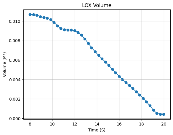
The information that we are using are basically the volume of LOX and Propane in the tanks
[3]:
# Define and set up LOX volume
lox_volume_liters = Function(
"../../data/rockets/berkeley/test124_Lox_Volume.csv",
extrapolation="zero",
inputs="Time (s)",
outputs="Volume (L)",
)
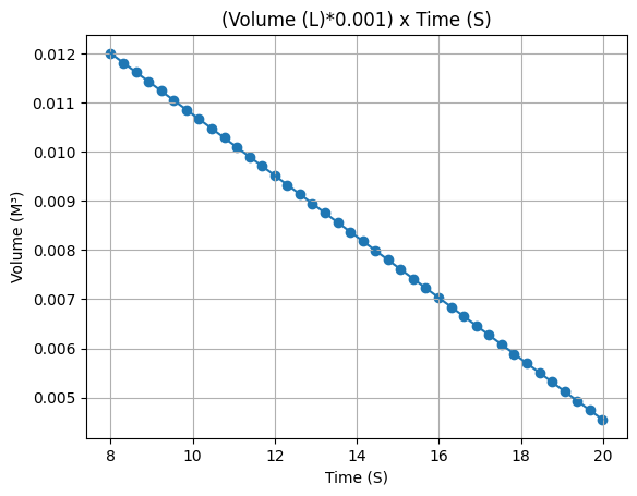
lox_volume = lox_volume_liters * 0.001 # Convert to m^3
lox_volume.set_discrete(8.003, 19.984, 40, interpolation="linear")
lox_volume.set_outputs("Volume (m³)")
lox_volume.set_title("LOX Volume")
# Plot LOX volume
lox_volume.plot(force_data=True)
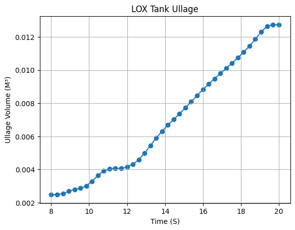
# Define and set up LOX tank ullage
lox_tank_ullage = 0.013167926436231077 - lox_volume
lox_tank_ullage.set_title("LOX Tank Ullage")
lox_tank_ullage.set_outputs("Ullage volume (m³)")
# Plot LOX tank ullage
lox_tank_ullage.plot(8, 20, force_data=True)
[4]:
# Define and set up Propane volume
propane_volume_liters = Function(
"../../data/rockets/berkeley/test124_Propane_Volume.csv",
inputs="Time (s)",
outputs="Volume (L)",
)
propane_volume = propane_volume_liters * 0.001 # Convert to m^3
propane_volume.set_discrete(8.003, 19.984, 40, interpolation="linear")
propane_volume.set_outputs("Volume (m³)")
# Plot Propane volume
propane_volume.plot(force_data=True)
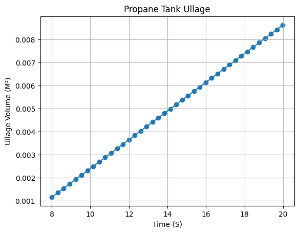
# Define and set up Propane tank ullage
propane_tank_ullage = 0.013167926436231077 - propane_volume
propane_tank_ullage.set_title("Propane Tank Ullage")
propane_tank_ullage.set_outputs("Ullage volume (m³)")
# Plot Propane tank ullage
propane_tank_ullage.plot(force_data=True)
Fluids#
Now it’s time to define the fluids that we are going to use in the simulation.
[5]:
# Define fluids
lox = Fluid(name="LOX", density=1024)
propane = Fluid(name="Propane", density=566)

# Define pressurizing gases with their respective pressures
lox_tank_pressurizing_gas = Fluid(name="N2", density=31.3 / 28)  # 450 PSI
propane_tank_pressurizing_gas = Fluid(
    name="N2", density=313 * 300 / 4500 / 28
)  # 300 PSI
pressurizing_gas = Fluid(name="N2", density=300)  # 4500 PSI
Tanks#
After the fluids, it is time to define all the 3 tanks that we have in the motor.
LOX Tank#
We first start defining the tank geometry, which is a cylinder with a spherical head.
[6]:
lox_tank_geometry = CylindricalTank(0.0744, 0.8068, spherical_caps=True)
Warning: Adding spherical caps to the tank will not modify the total height of the tank 0.8068 m. Its cylindrical portion height will be reduced to 0.6579999999999999 m.
Next, we use the tank geometry to define the tank itself.
[7]:
lox_tank = UllageBasedTank(
    name="LOX Tank",
    flux_time=(8, 20),
    geometry=lox_tank_geometry,
    gas=lox_tank_pressurizing_gas,
    liquid=lox,
    ullage=lox_tank_ullage,
)
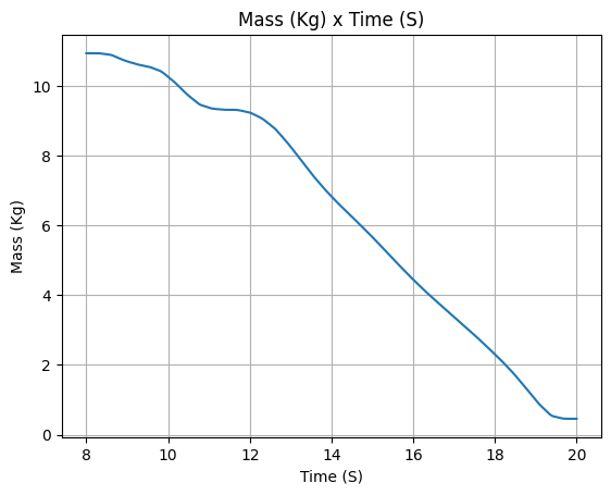
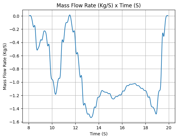
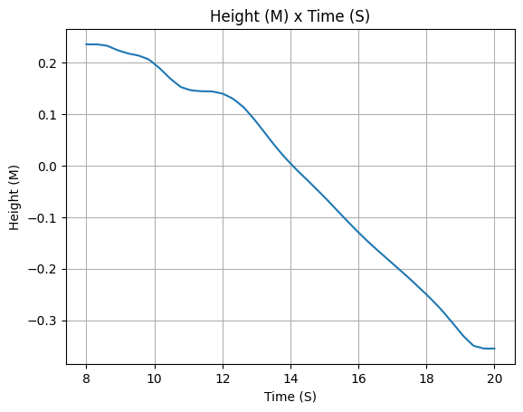
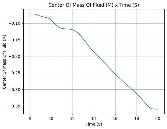
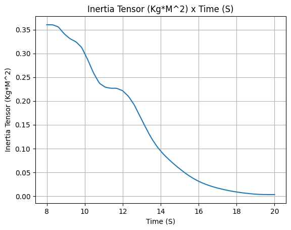
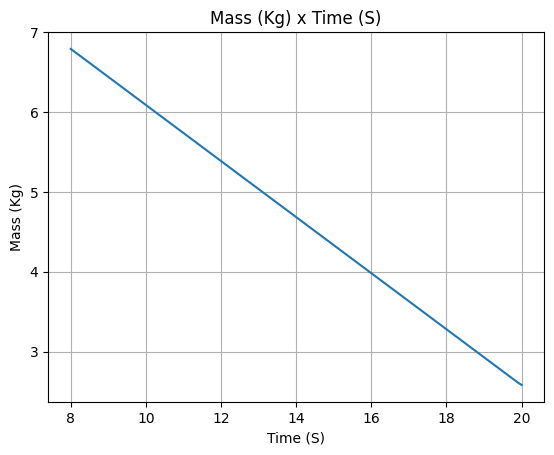
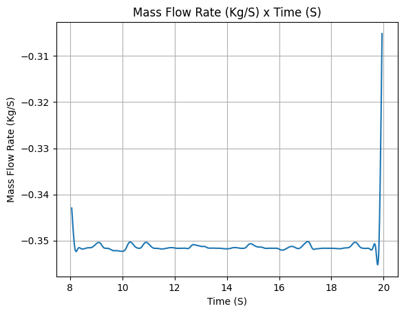
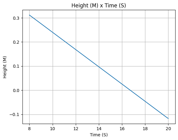
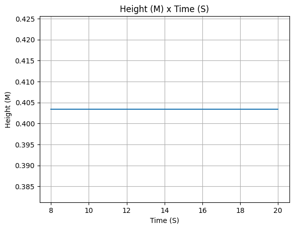
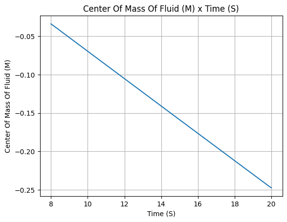
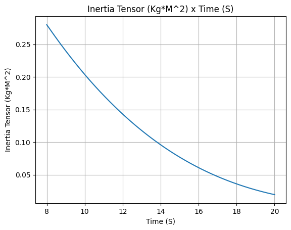
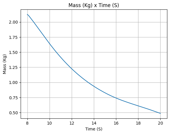
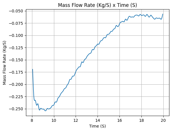
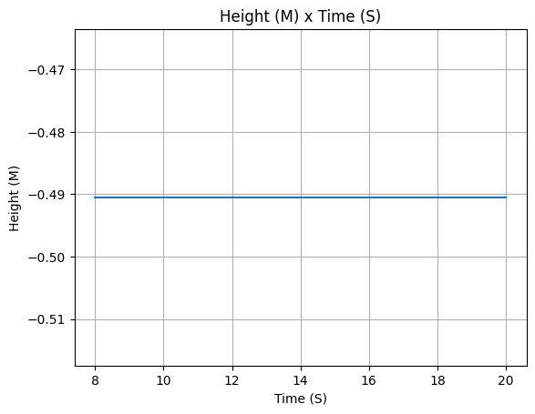
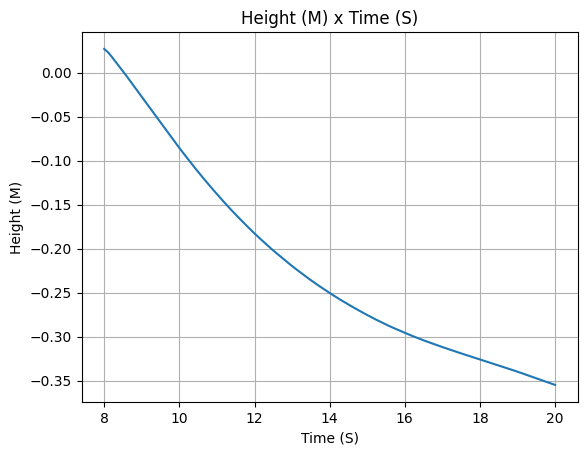
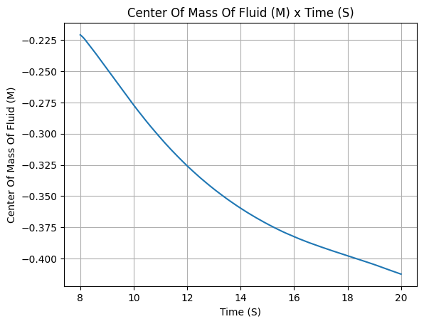
After defining, we stop for a minute to appreciate the evolution of mass and mass flow rate that were calculated by RocketPy.
Isn’t it beautiful?
[8]:
lox_tank.fluid_mass()
lox_tank.net_mass_flow_rate()
lox_tank.liquid_height()
lox_tank.gas_height()
lox_tank.center_of_mass()
lox_tank.inertia()

Propane Tank#
Our setup work is not done yet. We still need to define the propane tank, Which is a cylinder with a spherical head.
The propane has the role of pressurizing the LOX tank.
[9]:
propane_tank_geometry = CylindricalTank(0.0744, 0.8068, spherical_caps=True)
Warning: Adding spherical caps to the tank will not modify the total height of the tank 0.8068 m. Its cylindrical portion height will be reduced to 0.6579999999999999 m.
[10]:
propane_tank = UllageBasedTank(
    name="Propane Tank",
    flux_time=(8, 20),
    geometry=propane_tank_geometry,
    gas=propane_tank_pressurizing_gas,
    liquid=propane,
    ullage=propane_tank_ullage,
)
Again, let’s visualize the partial results.
[11]:
propane_tank.fluid_mass()
propane_tank.net_mass_flow_rate()
propane_tank.liquid_height()
propane_tank.gas_height()
propane_tank.center_of_mass()
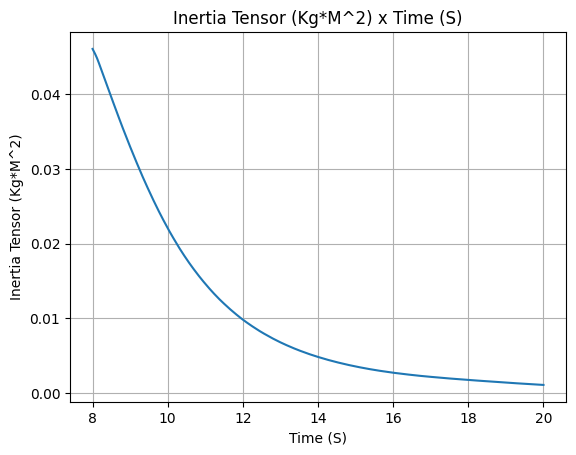
propane_tank.inertia()
Pressure Tank#
The third tank is the pressure tank, which is a cylinder with a spherical head.
[12]:
pressure_tank_geometry = CylindricalTank(0.135 / 2, 0.981, spherical_caps=True)
Warning: Adding spherical caps to the tank will not modify the total height of the tank 0.981 m. Its cylindrical portion height will be reduced to 0.846 m.
[13]:
pressure_tank = MassBasedTank(
    name="Pressure Tank",
    geometry=pressure_tank_geometry,
    liquid_mass=0,
    flux_time=(8, 20),
    gas_mass="../../data/rockets/berkeley/pressurantMassFiltered.csv",
    gas=pressurizing_gas,
    liquid=pressurizing_gas,
)
[14]:
pressure_tank.fluid_mass()
pressure_tank.net_mass_flow_rate()
pressure_tank.liquid_height()
pressure_tank.gas_height()
pressure_tank.center_of_mass()
pressure_tank.inertia()
Liquid Motor#
After defining the three tanks, we can finally define the liquid motor object, just check how simple it is!
[15]:
liquid_motor = LiquidMotor(
    thrust_source="../../data/rockets/berkeley/test124_Thrust_Curve.csv",
    center_of_dry_mass_position=0,
    dry_inertia=(0, 0, 0),
    dry_mass=0,
    burn_time=(8, 20),
    nozzle_radius=0.069 / 2,
    nozzle_position=-1.364,
    coordinate_system_orientation="nozzle_to_combustion_chamber",
)

liquid_motor.add_tank(propane_tank, position=-0.6446)
liquid_motor.add_tank(lox_tank, position=1.1144)
liquid_motor.add_tank(pressure_tank, position=2.4975)
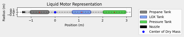
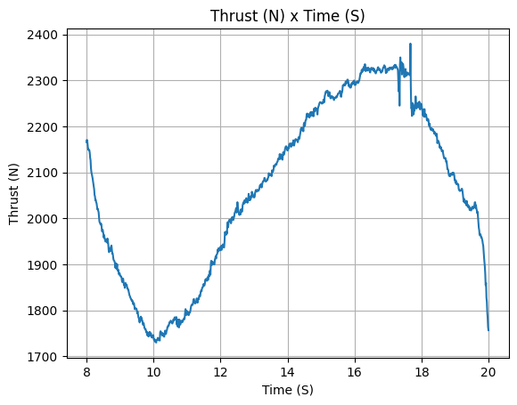
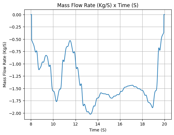
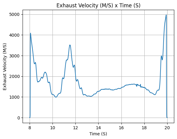
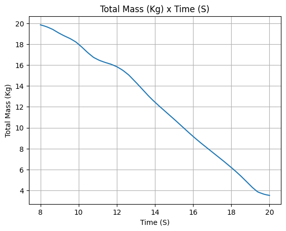
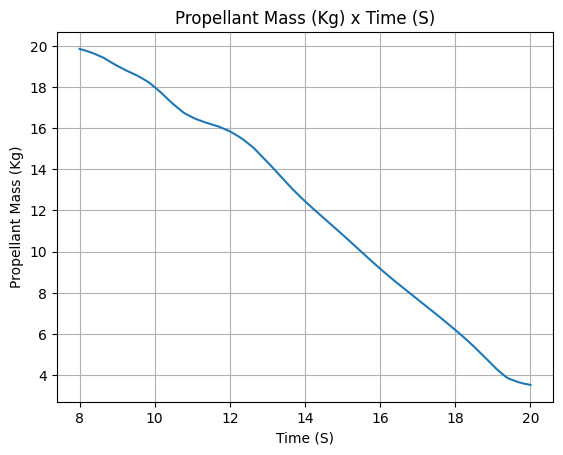
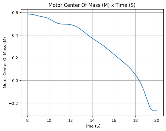
After defining it, we can check all the important information about the motor, such as the thrust curve, the mass flow rate curve, the specific impulse curve, and the burn time.
[16]:
liquid_motor.all_info()
Nozzle Details
Nozzle Radius: 0.0345 m

Motor Details
Total Burning Time: 12 s
Total Propellant Mass: 19.852 kg
Average Propellant Exhaust Velocity: 1697.621 m/s
Average Thrust: 2064.885 N
Maximum Thrust: 2428.4243134124745 N at 17.666 s after ignition.
Total Impulse: 24778.624 Ns
Rocket Definition#
The motor is ready to go, but we still need to define the rocket itself. Let’s see how it is done:
[17]:
berkeley_rocket = Rocket(
    radius=0.098,
    mass=63.4,
    inertia=(25, 25, 1),
    power_off_drag="../../data/rockets/berkeley/drag.csv",
    power_on_drag="../../data/rockets/berkeley/drag.csv",
    center_of_mass_without_motor=3.23,
    coordinate_system_orientation="nose_to_tail",
)
berkeley_rocket.add_motor(liquid_motor, position=4.2)
nose = berkeley_rocket.add_nose(length=0.7, kind="vonKarman", position=0)
tail = berkeley_rocket.add_tail(
    top_radius=0.098, bottom_radius=0.058, length=0.198, position=5.69 - 0.198
)

fins = berkeley_rocket.add_trapezoidal_fins(
    n=4,
    root_chord=0.355,
    tip_chord=0.0803,
    span=0.156,
    position=5.25,
    cant_angle=0,
)
[18]:
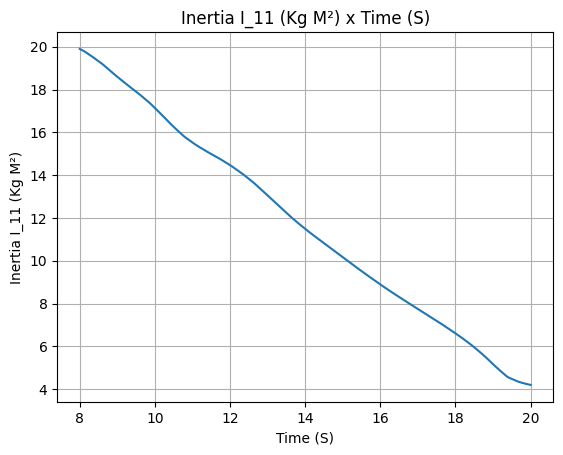
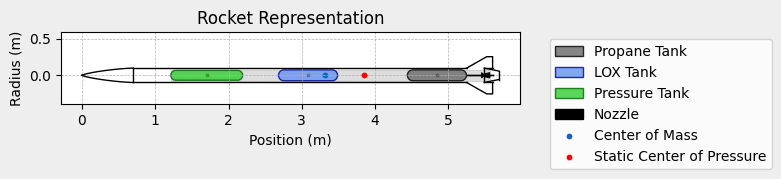
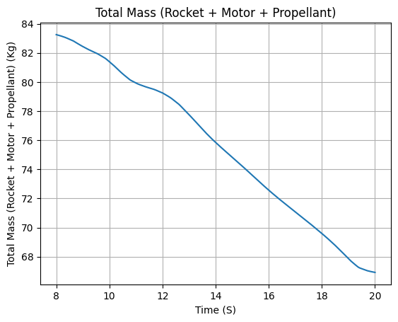
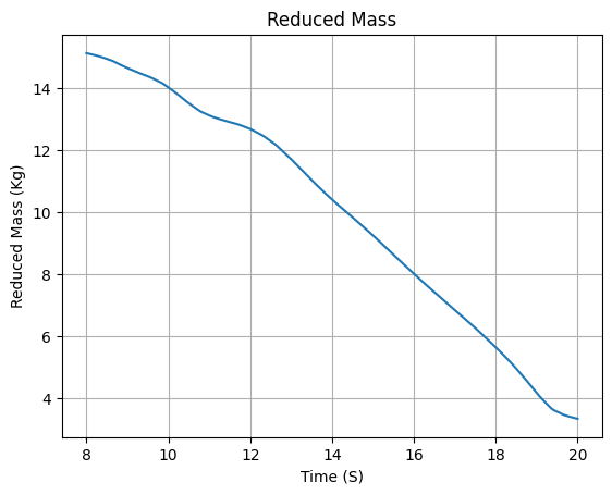
berkeley_rocket.all_info()
Inertia Details

Rocket Mass: 63.400 kg (without motor)
Rocket Dry Mass: 63.400 kg (with unloaded motor)
Rocket Loaded Mass: 83.252 kg
Rocket Inertia (with unloaded motor) 11: 25.000 kg*m2
Rocket Inertia (with unloaded motor) 22: 25.000 kg*m2
Rocket Inertia (with unloaded motor) 33: 1.000 kg*m2
Rocket Inertia (with unloaded motor) 12: 0.000 kg*m2
Rocket Inertia (with unloaded motor) 13: 0.000 kg*m2
Rocket Inertia (with unloaded motor) 23: 0.000 kg*m2

Geometrical Parameters

Rocket Maximum Radius: 0.098 m
Rocket Frontal Area: 0.030172 m2

Rocket Distances
Rocket Center of Dry Mass - Center of Mass without Motor: 0.000 m
Rocket Center of Dry Mass - Nozzle Exit: 2.334 m
Rocket Center of Dry Mass - Center of Propellant Mass: 0.384 m
Rocket Center of Mass - Rocket Loaded Center of Mass: 0.092 m


Aerodynamics Lift Coefficient Derivatives

Nose Cone Lift Coefficient Derivative: 2.000/rad
Tail Lift Coefficient Derivative: -1.299/rad
Fins Lift Coefficient Derivative: 5.895/rad

Center of Pressure

Nose Cone Center of Pressure position: 0.350 m
Tail Center of Pressure position: 5.583 m
Fins Center of Pressure position: 5.420 m

Stability

Center of Mass position (time=0): 3.322 m
Center of Pressure position (time=0): 3.851 m
Initial Static Margin (mach=0, time=0): 2.699 c
Final Static Margin (mach=0, time=burn_out): 2.834 c
Rocket Center of Mass (time=0) - Center of Pressure (mach=0): 0.529 m


Rocket Draw
----------------------------------------
Mass Plots
----------------------------------------
Aerodynamics Plots
----------------------------------------
Drag Plots
--------------------
Stability Plots
--------------------

Thrust-to-Weight Plot
----------------------------------------
Environment#
I swear this is the last step before actually flying the rocket. We need to define the environment in which the rocket will fly.
[19]:
env = Environment(latitude=35.347122986338356, longitude=-117.80893423073582)

env.set_date((2022, 12, 3, 14 + 7, 0, 0))  # UTC

env.set_atmospheric_model(
    type="custom_atmosphere",
    pressure=None,
    temperature=None,
    wind_u=[(0, 1), (500, 0), (1000, 5), (2500, 5.0), (5000, 10)],
    wind_v=[(0, 0), (500, 3), (1600, 2), (2500, -3), (5000, 10)],
)
[20]:
env.info()
Gravity Details

Acceleration of gravity at surface level:    9.7976 m/s²
Acceleration of gravity at  80.000 km (ASL): 9.5554 m/s²


Launch Site Details

Launch Date: 2022-12-03 21:00:00 UTC
Launch Site Latitude: 35.34712°
Launch Site Longitude: -117.80893°
Reference Datum: SIRGAS2000
Launch Site UTM coordinates: 426495.69 W    3911838.99 N
Launch Site UTM zone: 11S
Launch Site Surface Elevation: 0.0 m


Atmospheric Model Details

Atmospheric Model Type: custom_atmosphere
custom_atmosphere Maximum Height: 80.000 km

Surface Atmospheric Conditions

Surface Wind Speed: 1.00 m/s
Surface Wind Direction: 270.00°
Surface Wind Heading: 90.00°
Surface Pressure: 1013.25 hPa
Surface Temperature: 288.15 K
Surface Air Density: 1.225 kg/m³
Surface Speed of Sound: 340.29 m/s


Earth Model Details

Earth Radius at Launch site: 6371.02 km
Semi-major Axis: 6378.14 km
Semi-minor Axis: 6356.75 km
Flattening: 0.0034


Atmospheric Model Plots
Flight Simulation#
Finally, here we go with our flight simulation. We are going to run the simulation only until the apogee, since we are not interested in the landing phase.
The max_time_step parameter was set to a low value to ensure there won’t be any numerical instability during the launch rail phase.
[21]:
test_flight = Flight(
    rocket=berkeley_rocket,
    environment=env,
    rail_length=18.28,
    inclination=90,
    heading=23,
    max_time_step=0.1,
    terminate_on_apogee=True,
)
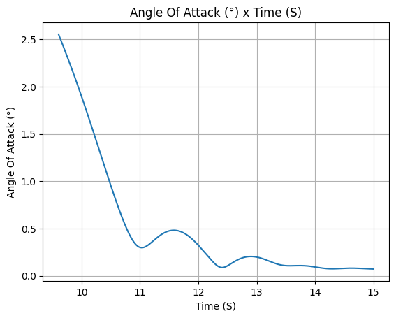
[22]:
test_flight.angle_of_attack.plot(test_flight.out_of_rail_time, 15)
[23]:
test_flight.all_info()
Initial Conditions
Initial time: 0.000 s
Position - x: 0.00 m | y: 0.00 m | z: 0.00 m
Velocity - Vx: 0.00 m/s | Vy: 0.00 m/s | Vz: 0.00 m/s
Attitude (quaternions) - e0: 0.980 | e1: 0.000 | e2: 0.000 | e3: -0.199
Euler Angles - Spin φ : -191.50° | Nutation θ: 0.00° | Precession ψ: 168.50°
Angular Velocity - ω1: 0.00 rad/s | ω2: 0.00 rad/s | ω3: 0.00 rad/s
Initial Stability Margin: 2.699 c
Surface Wind Conditions
Frontal Surface Wind Speed: 0.39 m/s
Lateral Surface Wind Speed: -0.92 m/s
Launch Rail
Launch Rail Length: 18.28 m
Launch Rail Inclination: 90.00°
Launch Rail Heading: 23.00°
Rail Departure State
Rail Departure Time: 9.604 s
Rail Departure Velocity: 21.742 m/s
Rail Departure Stability Margin: 2.697 c
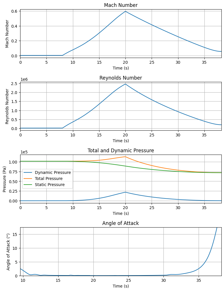
Rail Departure Angle of Attack: 2.554°
Rail Departure Thrust-Weight Ratio: 2.223
Rail Departure Reynolds Number: 2.916e+05
Burn out State
Burn out time: 20.000 s
Altitude at burn out: 1095.424 m (ASL) | 1095.424 m (AGL)
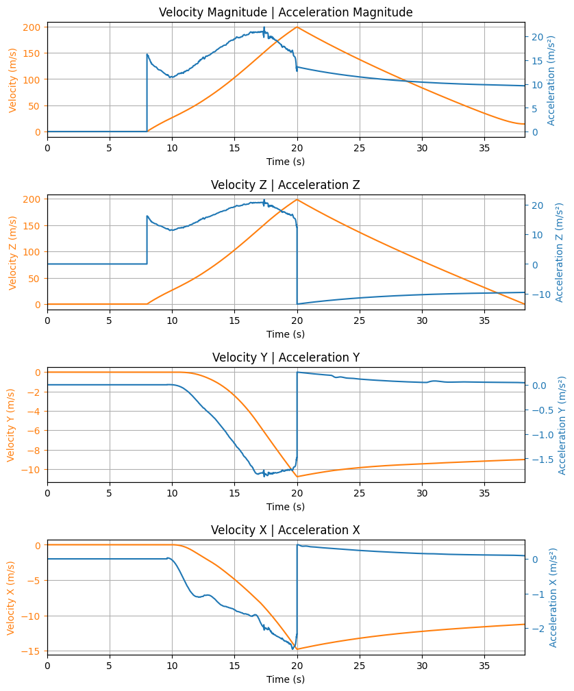
Rocket speed at burn out: 199.288 m/s
Freestream velocity at burn out: 199.890 m/s
Mach Number at burn out: 0.595
Kinetic energy at burn out: 1.329e+06 J
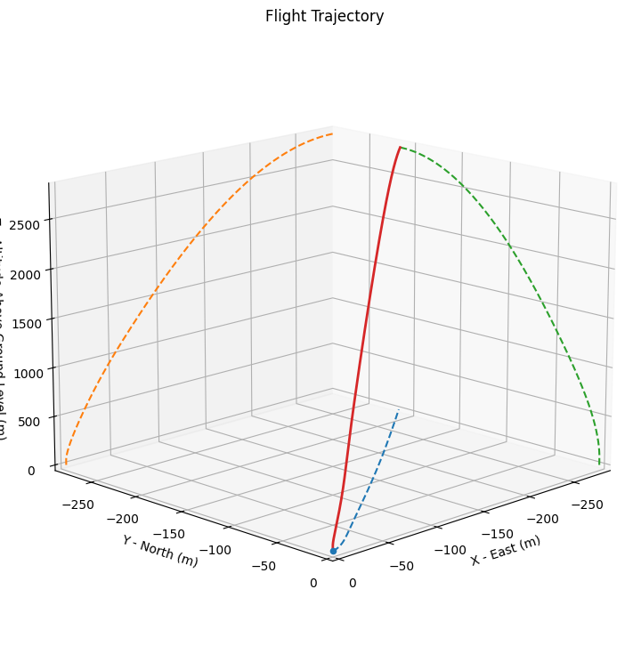
Apogee State
Apogee Time: 38.205 s
Apogee Altitude: 2801.341 m (ASL) | 2801.341 m (AGL)
Apogee Freestream Speed: 19.172 m/s
Apogee X position: -299.553 m
Apogee Y position: -218.811 m
Apogee latitude: 35.3451551°
Apogee longitude: -117.8122369°
Parachute Events
No Parachute Events Were Triggered.
Impact Conditions
Time of impact: 38.205 s
X impact: 0.000 m
Y impact: 0.000 m
Altitude impact: 2801.341 m (ASL) | 2801.341 m (AGL)
Latitude: 35.3451551°
Longitude: -117.8122369°
Vertical velocity at impact: 0.000 m/s
Number of parachutes triggered until impact: 0
Stability Margin
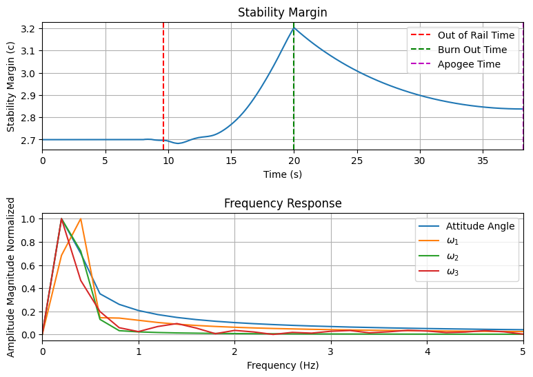
Initial Stability Margin: 2.699 c at 0.00 s
Out of Rail Stability Margin: 2.697 c at 9.60 s
Maximum Stability Margin: 3.203 c at 20.00 s
Minimum Stability Margin: 2.682 c at 10.80 s
Maximum Values
Maximum Speed: 199.288 m/s at 20.00 s
Maximum Mach Number: 0.595 Mach at 20.00 s
Maximum Reynolds Number: 2.461e+06 at 20.00 s
Maximum Dynamic Pressure: 2.200e+04 Pa at 20.00 s
Maximum Acceleration During Motor Burn: 21.461 m/s² at 17.37 s
Maximum Gs During Motor Burn: 2.188 g at 17.37 s
Maximum Acceleration After Motor Burn: 0.000 m/s² at 0.00 s
Maximum Gs After Motor Burn: 0.000 Gs at 0.00 s
Maximum Stability Margin: 3.203 c at 20.00 s
Numerical Integration Settings
Maximum Allowed Flight Time: 600.00 s
Maximum Allowed Time Step: 0.10 s
Minimum Allowed Time Step: 0.00e+00 s
Relative Error Tolerance: 1e-06
Absolute Error Tolerance: [0.001, 0.001, 0.001, 0.001, 0.001, 0.001, 1e-06, 1e-06, 1e-06, 1e-06, 0.001, 0.001, 0.001]
Allow Event Overshoot: True
Terminate Simulation on Apogee: True
Number of Time Steps Used: 694
Number of Derivative Functions Evaluation: 1497
Average Function Evaluations per Time Step: 2.157
Trajectory 3d Plot
Trajectory Kinematic Plots
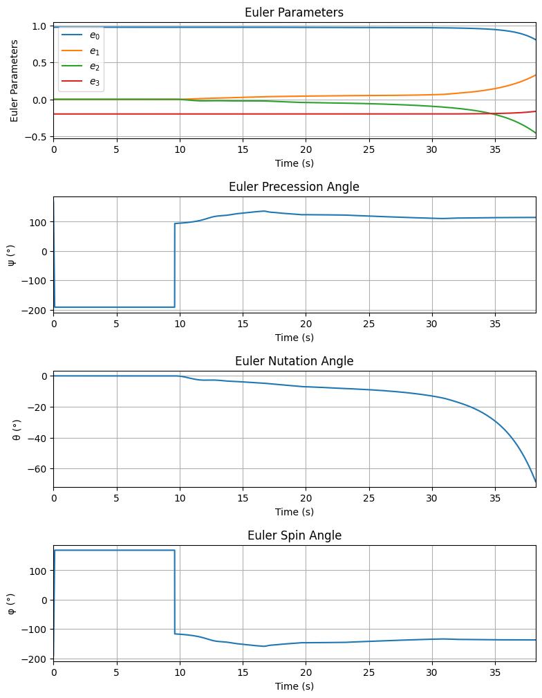
Angular Position Plots
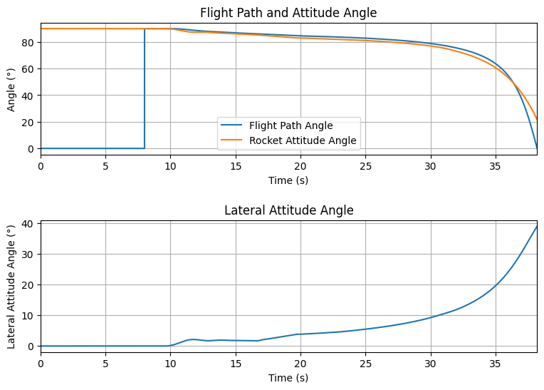
Path, Attitude and Lateral Attitude Angle plots
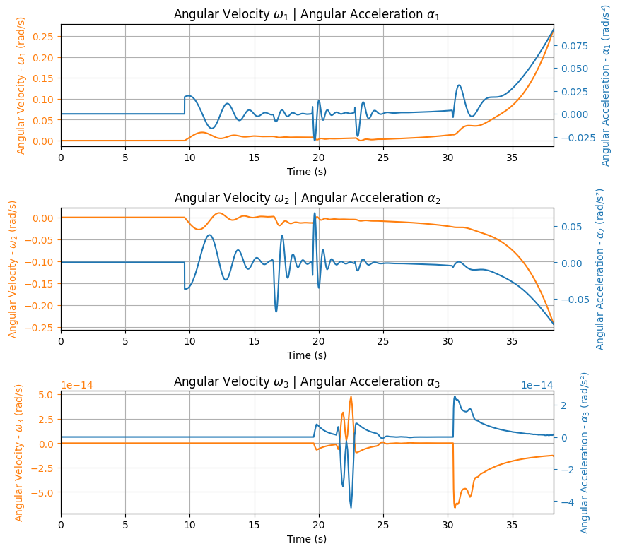
Trajectory Angular Velocity and Acceleration Plots
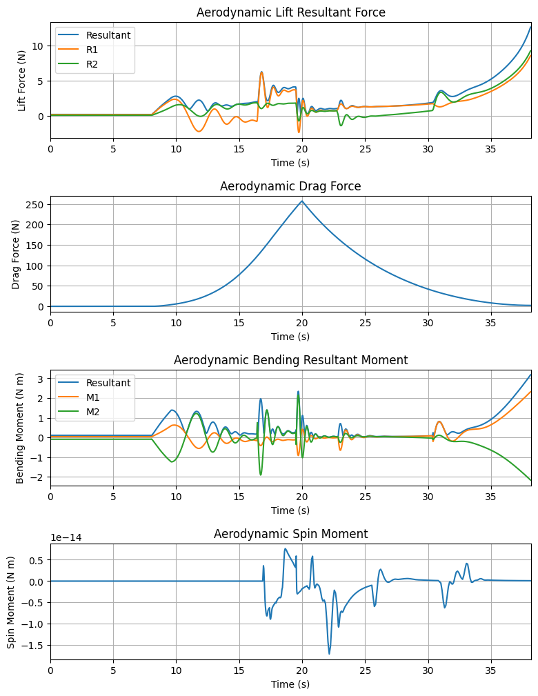
Aerodynamic Forces Plots
Rail Buttons Forces Plots
No rail buttons were defined. Skipping rail button plots.
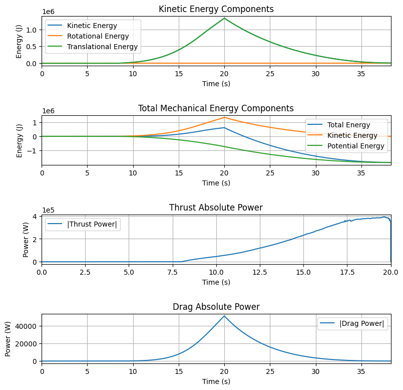
Trajectory Energy Plots
Trajectory Fluid Mechanics Plots
Trajectory Stability and Control Plots
Rocket and Parachute Pressure Plots
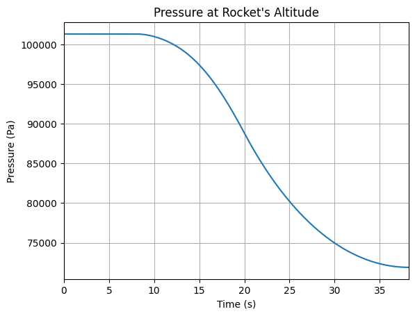
Rocket has no parachutes. No parachute plots available