Flight Class Usage#
The rocketpy.Flight class is the heart of RocketPy’s simulation engine.
It takes a rocketpy.Rocket, an rocketpy.Environment, and
launch parameters to simulate the complete flight trajectory of a rocket from
launch to landing.
See also
For a complete example of Flight simulation, see the First Simulation guide.
Creating a Flight Simulation#
Basic Flight Creation#
The most basic way to create a Flight simulation requires three mandatory parameters: a rocket, an environment, and a rail length.
from rocketpy import Environment, SolidMotor, Rocket, Flight

# Assuming you have already defined env, motor, and rocket objects
# (See Environment, Motor, and Rocket documentation for details)

# Create a basic flight
flight = Flight(
    rocket=rocket,           # Your Rocket object
    environment=env,         # Your Environment object
    rail_length=5.2,         # Length of launch rail in meters
)
Once created, the Flight object automatically runs the simulation and stores all results internally.
Launch Parameters#
You can customize the launch conditions by specifying additional parameters:
flight_custom = Flight(
    rocket=rocket,
    environment=env,
    rail_length=5.2,
    inclination=85,          # Rail inclination angle (degrees from horizontal)
    heading=90,              # Launch direction (degrees from North)
)
Key Launch Parameters:
inclination: Rail inclination angle relative to ground (0° = horizontal, 90° = vertical)
heading: Launch direction in degrees from North (0° = North, 90° = East, 180° = South, 270° = West)
Understanding Flight Parameters#
Coordinate Systems and Positioning#
RocketPy uses a launch-centered coordinate system:
X-axis: Points East (positive values = East direction)
Y-axis: Points North (positive values = North direction)
Z-axis: Points upward (positive values = altitude above launch site)
The rocket’s position is tracked relative to the launch site throughout the flight.
Initial Conditions#
The Flight class automatically calculates appropriate initial conditions based on:
Rail inclination and heading angles
Rocket orientation (affected by rail button positions if present)
Environment conditions (wind, atmospheric properties)
You can also specify custom initial conditions by passing an initial_solution
array or another Flight object to continue from a previous state.
Custom Initial Solution Vector
The initial_solution parameter accepts a 14-element array defining the complete
initial state of the rocket:
initial_solution = [
    t_initial,    # Initial time (s)
    x_init,       # Initial X position - East coordinate (m)
    y_init,       # Initial Y position - North coordinate (m)
    z_init,       # Initial Z position - altitude above launch site (m)
    vx_init,      # Initial velocity in X direction - East (m/s)
    vy_init,      # Initial velocity in Y direction - North (m/s)
    vz_init,      # Initial velocity in Z direction - upward (m/s)
    e0_init,      # Initial Euler parameter 0 (quaternion scalar part)
    e1_init,      # Initial Euler parameter 1 (quaternion i component)
    e2_init,      # Initial Euler parameter 2 (quaternion j component)
    e3_init,      # Initial Euler parameter 3 (quaternion k component)
    w1_init,      # Initial angular velocity about rocket's x-axis (rad/s)
    w2_init,      # Initial angular velocity about rocket's y-axis (rad/s)
    w3_init       # Initial angular velocity about rocket's z-axis (rad/s)
]
Using a Previous Flight as Initial Condition
You can also continue a simulation from where another flight ended:
# Continue from the final state of a previous flight
continued_flight = Flight(
    rocket=rocket,
    environment=env,
    rail_length=0,  # Set to 0 when continuing from free flight
    initial_solution=flight  # Use previous Flight object
)
This is particularly useful for multi-stage simulations or when analyzing different scenarios from a specific flight condition.
Simulation Control Parameters#
Time Control:
max_time: Maximum simulation duration (default: 600 seconds)max_time_step: Maximum integration step size (default: infinity)min_time_step: Minimum integration step size (default: 0)
Note
These time control parameters can significantly help with integration stability in challenging simulation cases. This is particularly useful for liquid and hybrid motors, which often have more complex thrust curves and transient behaviors that can cause numerical integration difficulties.
Accuracy Control:
rtol: Relative tolerance for numerical integration (default: 1e-6)atol: Absolute tolerance for numerical integration (default: auto-calculated)
Note
Increasing the tolerance values can speed up simulations but may reduce accuracy.
Simulation Behavior:
terminate_on_apogee: Stop simulation at apogee (default: False)time_overshoot: Allow time step overshoot for efficiency (default: True)
Accessing Simulation Results#
Once a Flight simulation is complete, you can access a wealth of data about the rocket’s trajectory and performance.
Trajectory Data#
Basic position and velocity data:
# Position coordinates (as functions of time)
x_trajectory = flight.x          # East coordinate (m)
y_trajectory = flight.y          # North coordinate (m)
altitude = flight.z              # Altitude above launch site (m)

# Velocity components (as functions of time)
vx = flight.vx                   # East velocity (m/s)
vy = flight.vy                   # North velocity (m/s)
vz = flight.vz                   # Vertical velocity (m/s)

# Access specific values at given times
altitude_at_10s = flight.z(10)   # Altitude at t=10 seconds
max_altitude = flight.apogee     # Maximum altitude reached
Key Flight Events#
Important events during the flight:
# Rail departure
rail_departure_time = flight.out_of_rail_time
rail_departure_velocity = flight.out_of_rail_velocity

# Apogee
apogee_time = flight.apogee_time
apogee_altitude = flight.apogee
apogee_coordinates = (flight.apogee_x, flight.apogee_y)

# Landing/Impact
impact_time = flight.impact_state[0]
impact_velocity = flight.impact_velocity
impact_coordinates = (flight.x_impact, flight.y_impact)
Forces and Accelerations#
The Flight object provides access to all forces and accelerations acting on the rocket:
# Linear accelerations in inertial frame (m/s²)
ax = flight.ax                   # East acceleration
ay = flight.ay                   # North acceleration
az = flight.az                   # Vertical acceleration

# Aerodynamic forces in body frame (N)
R1 = flight.R1                   # X-axis aerodynamic force
R2 = flight.R2                   # Y-axis aerodynamic force
R3 = flight.R3                   # Z-axis aerodynamic force (drag)

# Aerodynamic moments in body frame (N⋅m)
M1 = flight.M1                   # Roll moment
M2 = flight.M2                   # Pitch moment
M3 = flight.M3                   # Yaw moment
Attitude and Orientation#
Rocket orientation throughout the flight:
# Euler parameters (quaternions)
e0, e1, e2, e3 = flight.e0, flight.e1, flight.e2, flight.e3

# Angular velocities in body frame (rad/s)
w1 = flight.w1                   # Roll rate
w2 = flight.w2                   # Pitch rate
w3 = flight.w3                   # Yaw rate

# Derived attitude angles
attitude_angle = flight.attitude_angle
path_angle = flight.path_angle
Performance Metrics#
Key performance indicators:
# Velocity and speed
total_speed = flight.speed
mach_number = flight.mach_number

# Stability indicators
static_margin = flight.static_margin
stability_margin = flight.stability_margin
Accessing Raw Simulation Data#
For users who need direct access to the raw numerical simulation results,
the Flight object provides the complete solution array through the solution
and solution_array attributes.
Flight.solution
The Flight.solution attribute contains the raw simulation data as a list of
state vectors, where each row represents the rocket’s complete state at a specific time:
# Access the raw solution list
raw_solution = flight.solution

# Each element is a 14-element state vector:
# [time, x, y, z, vx, vy, vz, e0, e1, e2, e3, w1, w2, w3]
initial_state = flight.solution[0]  # First time step
final_state = flight.solution[-1]   # Last time step

print(f"Initial state: {initial_state}")
print(f"Final state: {final_state}")
Initial state: [0, 0, 0, 1400, 0, 0, 0, np.float64(0.7044160264027587), np.float64(-0.06162841671621935), np.float64(0.061628416716219346), np.float64(-0.7044160264027586), 0, 0, 0]
Final state: [48.97534056388913, np.float64(2020.4103181023356), np.float64(-4.051220217150634), np.float64(1399.9999995346768), np.float64(25.065878130337143), np.float64(-0.1603702919865078), np.float64(-332.7495460496878), np.float64(0.7044160264027587), np.float64(-0.06162841671621935), np.float64(0.061628416716219346), np.float64(-0.7044160264027586), np.float64(0.0), np.float64(0.0), np.float64(0.0)]
Flight.solution_array
For easier numerical analysis, use solution_array which provides the same data
as a NumPy array:
import numpy as np

# Get solution as NumPy array for easier manipulation
solution_array = flight.solution_array  # Shape: (n_time_steps, 14)

# Extract specific columns (state variables)
time_array = solution_array[:, 0]        # Time values
position_data = solution_array[:, 1:4]   # X, Y, Z positions
velocity_data = solution_array[:, 4:7]   # Vx, Vy, Vz velocities
quaternions = solution_array[:, 7:11]    # e0, e1, e2, e3
angular_velocities = solution_array[:, 11:14]  # w1, w2, w3

# Example: Calculate velocity magnitude manually
velocity_magnitude = np.sqrt(np.sum(velocity_data**2, axis=1))
State Vector Format
Each row in the solution array follows this 14-element format:
[time, x, y, z, vx, vy, vz, e0, e1, e2, e3, w1, w2, w3]
- Where:
time: Simulation time in secondsx, y, z: Position coordinates in meters (East, North, Up)vx, vy, vz: Velocity components in m/s (East, North, Up)e0, e1, e2, e3: Euler parameters (quaternions) for attitudew1, w2, w3: Angular velocities in rad/s (body frame: roll, pitch, yaw rates)
Getting State at Specific Time
You can extract the rocket’s state at any specific time during the flight:
# Get complete state vector at t=10 seconds
state_at_10s = flight.get_solution_at_time(10.0)

print(f"State at t=10s: {state_at_10s}")

# Extract specific values from the state vector
time_10s = state_at_10s[0]
altitude_10s = state_at_10s[3]  # Z coordinate
speed_10s = np.sqrt(state_at_10s[4]**2 + state_at_10s[5]**2 + state_at_10s[6]**2)

print(f"At t={time_10s}s: altitude={altitude_10s:.1f}m, speed={speed_10s:.1f}m/s")
State at t=10s: [ 1.02810622e+01  4.40332604e+02 -1.57704770e-01  3.42776162e+03
  4.60657180e+01 -3.48953672e-02  1.66134356e+02  7.04416026e-01
 -6.16284167e-02  6.16284167e-02 -7.04416026e-01  0.00000000e+00
  0.00000000e+00  0.00000000e+00]
At t=10.281062192923857s: altitude=3427.8m, speed=172.4m/s
This raw data access is particularly useful for:
Custom post-processing and analysis
Exporting data to external tools
Implementing custom flight metrics
Monte Carlo analysis and statistical studies
Integration with other simulation frameworks
Plotting Flight Data#
The Flight class provides comprehensive plotting capabilities through the
plots attribute.
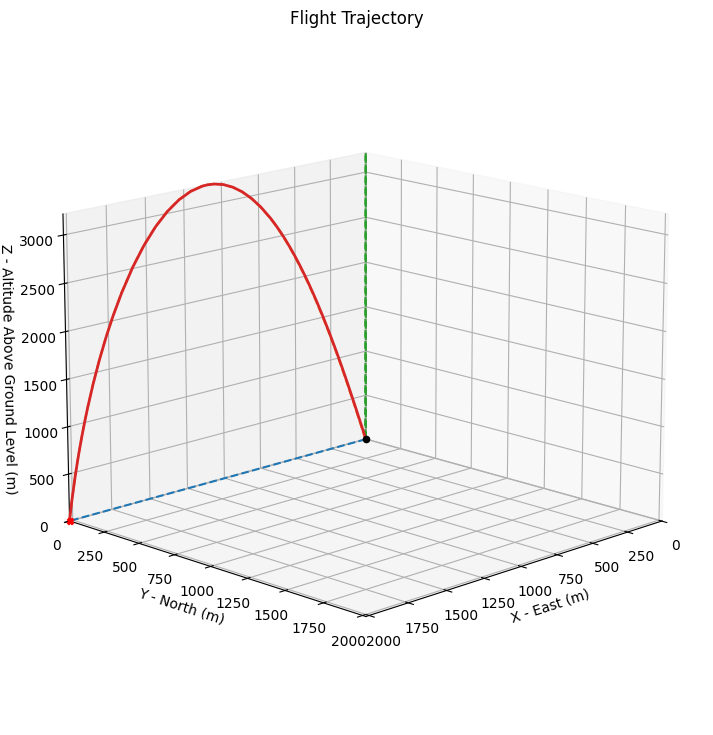
Trajectory Visualization#
# 3D trajectory plot
flight.plots.trajectory_3d()

# 2D trajectory (ground track)
flight.plots.linear_kinematics_data()
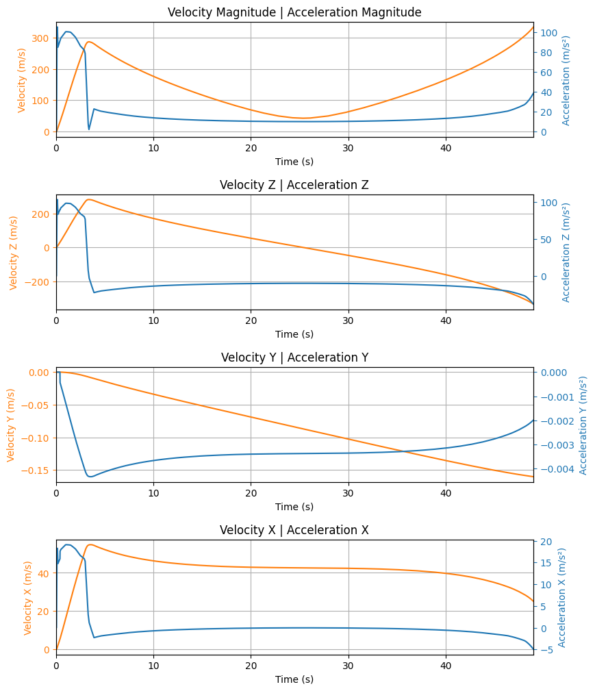
Flight Data Plots#
# Velocity and acceleration plots
flight.plots.linear_kinematics_data()
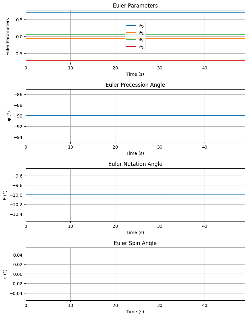
# Attitude and angular motion
flight.plots.attitude_data()
flight.plots.angular_kinematics_data()
# Flight path and orientation
flight.plots.flight_path_angle_data()
Forces and Moments#
# Aerodynamic forces
flight.plots.aerodynamic_forces()

# Rail button forces (if applicable)
flight.plots.rail_buttons_forces()
Energy Analysis#
# Energy plots
flight.plots.energy_data()
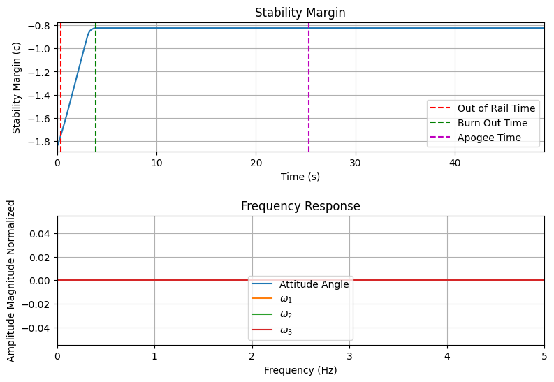
# Stability analysis
flight.plots.stability_and_control_data()
Comprehensive Analysis#
For a complete overview of all plots:
# Show all available plots
flight.all_info()
Initial Conditions

Initial time: 0.000 s
Position - x: 0.00 m | y: 0.00 m | z: 1400.00 m
Velocity - Vx: 0.00 m/s | Vy: 0.00 m/s | Vz: 0.00 m/s
Attitude (quaternions) - e0: 0.704 | e1: -0.062 | e2: 0.062 | e3: -0.704
Euler Angles - Spin φ : 0.00° | Nutation θ: -10.00° | Precession ψ: -90.00°
Angular Velocity - ω1: 0.00 rad/s | ω2: 0.00 rad/s | ω3: 0.00 rad/s
Initial Stability Margin: -1.836 c


Surface Wind Conditions

Frontal Surface Wind Speed: 0.00 m/s
Lateral Surface Wind Speed: 0.00 m/s


Launch Rail

Launch Rail Length: 5.2 m
Launch Rail Inclination: 80.00°
Launch Rail Heading: 90.00°


Rail Departure State

Rail Departure Time: 0.415 s
Rail Departure Velocity: 30.492 m/s
Rail Departure Stability Margin: -1.742 c
Rail Departure Angle of Attack: 0.000°
Rail Departure Thrust-Weight Ratio: 10.303
Rail Departure Reynolds Number: 2.373e+05


Burn out State

Burn out time: 3.900 s
Altitude at burn out: 2049.776 m (ASL) | 649.776 m (AGL)
Rocket speed at burn out: 280.008 m/s
Freestream velocity at burn out: 280.008 m/s
Mach Number at burn out: 0.844
Kinetic energy at burn out: 6.367e+05 J


Apogee State

Apogee Time: 25.344 s
Apogee Altitude: 4616.176 m (ASL) | 3216.176 m (AGL)
Apogee Freestream Speed: 42.595 m/s
Apogee X position: 1096.634 m
Apogee Y position: -1.080 m
Apogee latitude: 32.9902437°
Apogee longitude: -106.9632414°


Parachute Events

No Parachute Events Were Triggered.


Impact Conditions

Time of impact: 48.975 s
X impact: 2020.410 m
Y impact: -4.051 m
Altitude impact: 1400.000 m (ASL) | -0.000 m (AGL)
Latitude: 32.9902157°
Longitude: -106.9533380°
Vertical velocity at impact: -332.750 m/s
Number of parachutes triggered until impact: 0


Stability Margin

Initial Stability Margin: -1.836 c at 0.00 s
Out of Rail Stability Margin: -1.742 c at 0.41 s
Maximum Stability Margin: -0.825 c at 3.90 s
Minimum Stability Margin: -1.836 c at 0.00 s


Maximum Values

Maximum Speed: 333.692 m/s at 48.98 s
Maximum Mach Number: 0.997 Mach at 48.98 s
Maximum Reynolds Number: 2.599e+06 at 48.98 s
Maximum Dynamic Pressure: 5.949e+04 Pa at 48.98 s
Maximum Acceleration During Motor Burn: 105.172 m/s² at 0.15 s
Maximum Gs During Motor Burn: 10.725 g at 0.15 s
Maximum Acceleration After Motor Burn: 38.547 m/s² at 48.98 s
Maximum Gs After Motor Burn: 3.931 Gs at 48.98 s
Maximum Stability Margin: -0.825 c at 3.90 s


Numerical Integration Settings

Maximum Allowed Flight Time: 600.00 s
Maximum Allowed Time Step: inf s
Minimum Allowed Time Step: 0.00e+00 s
Relative Error Tolerance: 1e-06
Absolute Error Tolerance: [0.001, 0.001, 0.001, 0.001, 0.001, 0.001, 1e-06, 1e-06, 1e-06, 1e-06, 0.001, 0.001, 0.001]
Allow Event Overshoot: True
Terminate Simulation on Apogee: False
Number of Time Steps Used: 212
Number of Derivative Functions Evaluation: 406
Average Function Evaluations per Time Step: 1.915


Trajectory 3d Plot
Trajectory Kinematic Plots
Angular Position Plots
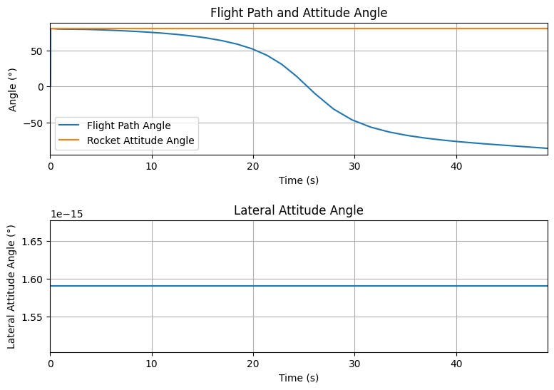
Path, Attitude and Lateral Attitude Angle plots
Trajectory Angular Velocity and Acceleration Plots
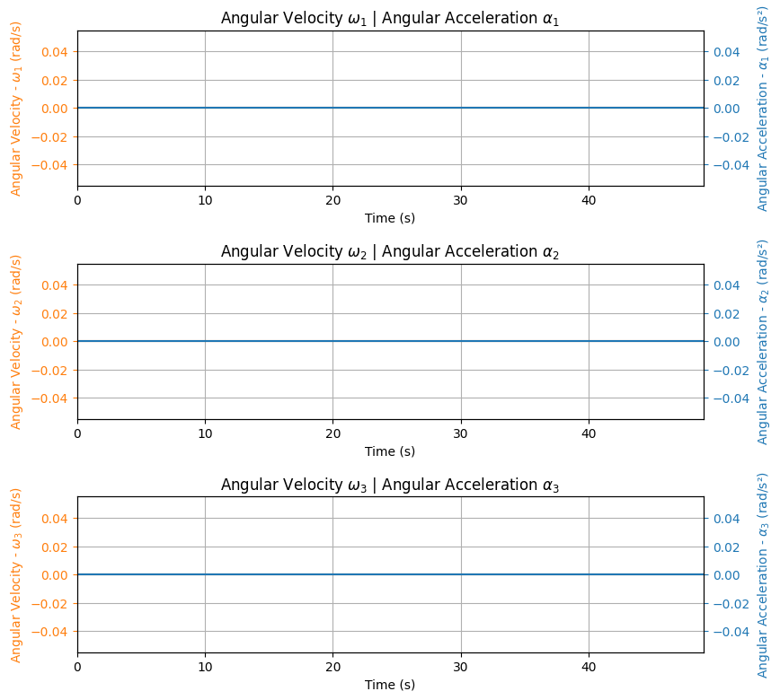
Aerodynamic Forces Plots
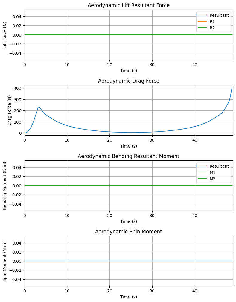
Rail Buttons Bending Moments Plots

No rail buttons were defined. Skipping rail button bending moment plots.


Rail Buttons Forces Plots

No rail buttons were defined. Skipping rail button plots.


Trajectory Energy Plots
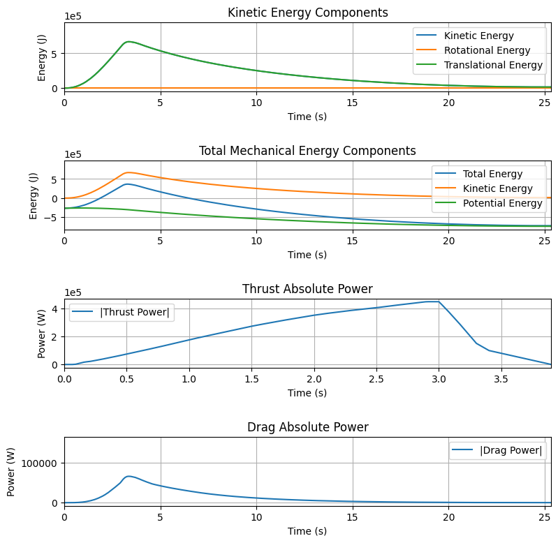
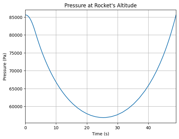
Trajectory Fluid Mechanics Plots
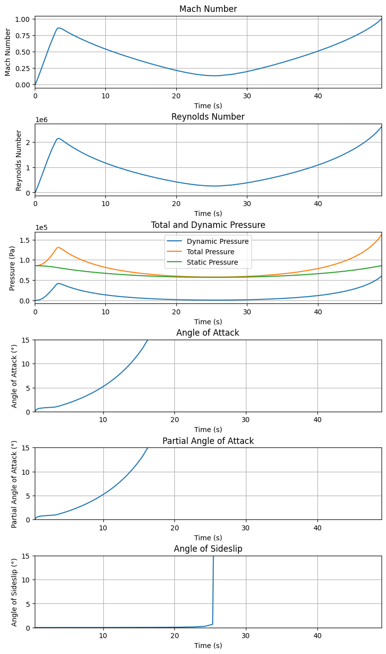
Trajectory Stability and Control Plots
Rocket and Parachute Pressure Plots
Rocket has no parachutes. No parachute plots available
Printing Flight Information#
The Flight class also provides detailed text output through the prints attribute.
Flight Summary#
# Complete flight information
flight.info()

# All detailed information
flight.all_info()
Specific Information Sections#
# Initial conditions
flight.prints.initial_conditions()

# Wind and environment conditions
flight.prints.surface_wind_conditions()

# Launch rail information
flight.prints.launch_rail_conditions()

# Rail departure conditions
flight.prints.out_of_rail_conditions()

# Motor burn out conditions
flight.prints.burn_out_conditions()

# Apogee conditions
flight.prints.apogee_conditions()

# Landing/impact conditions
flight.prints.impact_conditions()

# Maximum values during flight
flight.prints.maximum_values()
Advanced Features#
Custom Equations of Motion#
RocketPy supports different sets of equations of motion:
# Standard 6-DOF equations (default)
flight_6dof = Flight(
    rocket=rocket,
    environment=env,
    rail_length=5.2,
    equations_of_motion="standard"
)

# Simplified solid propulsion equations (legacy)
# This may run a bit faster with no accuracy loss, but only works for solid motors
flight_simple = Flight(
    rocket=rocket,
    environment=env,
    rail_length=5.2,
    equations_of_motion="solid_propulsion"
)
Integration Method Selection#
You can choose different numerical integration methods using the ode_solver parameter.
RocketPy supports the following integration methods from scipy.integrate.solve_ivp:
Available ODE Solvers:
‘LSODA’ (default): Recommended for most flights. Automatically switches between stiff and non-stiff methods
‘RK45’: Explicit Runge-Kutta method of order 5(4). Good for non-stiff problems
‘RK23’: Explicit Runge-Kutta method of order 3(2). Faster but less accurate than RK45
‘DOP853’: Explicit Runge-Kutta method of order 8. High accuracy for smooth problems
‘Radau’: Implicit Runge-Kutta method of order 5. Good for stiff problems
‘BDF’: Implicit multi-step variable-order method. Efficient for stiff problems
# High-accuracy integration (default, recommended for most cases)
flight_default = Flight(
    rocket=rocket,
    environment=env,
    rail_length=5.2,
    ode_solver="LSODA"
)

# Fast integration for quick simulations
flight_fast = Flight(
    rocket=rocket,
    environment=env,
    rail_length=5.2,
    ode_solver="RK45"
)

# Very high accuracy for smooth problems
flight_high_accuracy = Flight(
    rocket=rocket,
    environment=env,
    rail_length=5.2,
    ode_solver="DOP853"
)

# For stiff problems (e.g., complex motor thrust curves)
flight_stiff = Flight(
    rocket=rocket,
    environment=env,
    rail_length=5.2,
    ode_solver="BDF"
)
You can also pass a custom scipy.integrate.OdeSolver object for advanced use cases.
For more information on integration methods, see the scipy documentation.
Exporting Flight Data#
You can export flight data for external analysis:
# Convert to dictionary format
flight_data = flight.to_dict(include_outputs=True)
# NOTE: RocketPy offers an unofficial json serializer, see rocketpy._encoders for details
Common Issues and Solutions#
Integration Problems:
Reduce
max_time_stepfor more accuracyIncrease
rtolfor faster but less accurate simulationsCheck rocket and environment definitions for unrealistic values
Missing Events:
Ensure
max_timeis sufficient for complete flightVerify parachute trigger conditions
Check for premature termination conditions
You can set
verbose=Truein the Flight constructor to get detailed logs during simulation
Performance Issues:
Set
time_overshoot=Truefor better performanceUse simpler integration methods for quick runs
Consider reducing the complexity of atmospheric models