First Simulation with RocketPy#
Here we will show how to set up a complete simulation with RocketPy.
See also
You can find all the code used in this page in the notebooks folder of the RocketPy repository. You can also run the code in Google Colab:
RocketPy is structured into four main classes, each one with its own purpose:
Environment- Keeps data related to weather.Motor- Subdivided into SolidMotor, HybridMotor and LiquidMotor. Keeps data related to rocket motors.Rocket- Keeps data related to a rocket.Flight- Runs the simulation and keeps the results.
By using these four classes, we can create a complete simulation of a rocket flight.
The following image shows how the four main classes interact with each other to generate a rocket flight simulation:

Setting Up a Simulation#
A basic simulation with RocketPy is composed of the following steps:
Defining a
Environment,MotorandRocketobject.Running the simulation by defining a
Flightobject.Plotting/Analyzing the results.
Tip
It is recommended that RocketPy is ran in a Jupyter Notebook. This way, the results can be easily plotted and analyzed.
The first step to set up a simulation, we need to first import the classes we will use from RocketPy:
from rocketpy import Environment, SolidMotor, Rocket, Flight
Note
Here we will use a SolidMotor as an example, but the same steps can be applied to Hybrid and Liquid motors.
Defining a Environment#
The Environment class is used to store data related to the weather and the
wind conditions of the launch site. The weather conditions are imported from
weather organizations such as NOAA and ECMWF.
To define a Environment object, we need to first specify some information regarding the launch site:
env = Environment(latitude=32.990254, longitude=-106.974998, elevation=1400)
Next, we need to specify the atmospheric model to be used. In this example, we will get GFS forecasts data from tomorrow.
First we must set the date of the simulation. The date must be given in a tuple
with the following format: (year, month, day, hour).
The hour is given in UTC time. Here we use the datetime library to get the date
of tomorrow:
import datetime

tomorrow = datetime.date.today() + datetime.timedelta(days=1)

env.set_date(
    (tomorrow.year, tomorrow.month, tomorrow.day, 12)
)  # Hour given in UTC time
env.set_atmospheric_model(type="Forecast", file="GFS")
See also
To learn more about the different types of atmospheric models and a better description of the initialization parameters, see Environment Usage.
We can see what the weather will look like by calling the info method:
env.info()
Gravity Details

Acceleration of gravity at surface level:    9.7911 m/s²
Acceleration of gravity at  79.016 km (ASL): 9.5563 m/s²


Launch Site Details

Launch Date: 2026-07-14 12:00:00 UTC
Launch Site Latitude: 32.99025°
Launch Site Longitude: -106.97500°
Reference Datum: SIRGAS2000
Launch Site UTM coordinates: 315468.64 W    3651938.65 N
Launch Site UTM zone: 13S
Launch Site Surface Elevation: 1471.5 m


Atmospheric Model Details

Atmospheric Model Type: Forecast
Forecast Maximum Height: 79.016 km
Forecast Time Period: from 2026-07-07 00:00:00 to 2026-07-29 18:00:00 utc
Forecast Hour Interval: 3 hrs
Forecast Latitude Range: From 90.0° to -90.0°
Forecast Longitude Range: From 0.0° to 359.75°

Surface Atmospheric Conditions

Surface Wind Speed: 0.43 m/s
Surface Wind Direction: 84.06°
Surface Wind Heading: 264.06°
Surface Pressure: 856.95 hPa
Surface Temperature: 296.83 K
Surface Air Density: 1.006 kg/m³
Surface Speed of Sound: 345.38 m/s


Earth Model Details

Earth Radius at Launch site: 6371.83 km
Semi-major Axis: 6378.14 km
Semi-minor Axis: 6356.75 km
Flattening: 0.0034


Atmospheric Model Plots
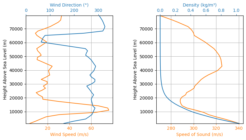
Defining a Motor#
RocketPy can simulate Solid, Hybrid and Liquid motors. Each type of
motor has its own class: rocketpy.SolidMotor,
rocketpy.HybridMotor and rocketpy.LiquidMotor.
In this example, we will use a SolidMotor. To define a SolidMotor, we need
to specify several parameters:
Pro75M1670 = SolidMotor(
    thrust_source="../data/motors/cesaroni/Cesaroni_M1670.eng",
    dry_mass=1.815,
    dry_inertia=(0.125, 0.125, 0.002),
    nozzle_radius=33 / 1000,
    grain_number=5,
    grain_density=1815,
    grain_outer_radius=33 / 1000,
    grain_initial_inner_radius=15 / 1000,
    grain_initial_height=120 / 1000,
    grain_separation=5 / 1000,
    grains_center_of_mass_position=0.397,
    center_of_dry_mass_position=0.317,
    nozzle_position=0,
    burn_time=3.9,
    throat_radius=11 / 1000,
    coordinate_system_orientation="nozzle_to_combustion_chamber",
)
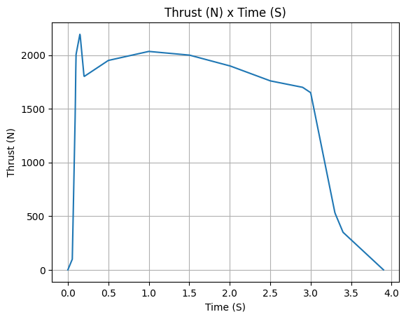
Pro75M1670.info()
Nozzle Details
Nozzle Radius: 0.033 m
Nozzle Throat Radius: 0.011 m

Grain Details
Number of Grains: 5
Grain Spacing: 0.005 m
Grain Density: 1815 kg/m3
Grain Outer Radius: 0.033 m
Grain Inner Radius: 0.015 m
Grain Height: 0.12 m
Grain Volume: 0.000 m3
Grain Mass: 0.591 kg

Motor Details
Total Burning Time: 3.9 s
Total Propellant Mass: 2.956 kg
Structural Mass Ratio: 0.380
Average Propellant Exhaust Velocity: 2038.745 m/s
Average Thrust: 1545.218 N
Maximum Thrust: 2200.0 N at 0.15 s after ignition.
Total Impulse: 6026.350 Ns
Defining a Rocket#
To create a complete Rocket object, we need to complete some steps:
Define the rocket itself by passing in the rocket’s dry mass, inertia, drag coefficient and radius;
Add a motor;
Add, if desired, aerodynamic surfaces;
Add, if desired, parachutes;
Set, if desired, rail guides;
See results.
See also
To learn more about each step, see Rocket Class Usage
To create a Rocket object, we need to specify some parameters.
calisto = Rocket(
    radius=127 / 2000,
    mass=14.426,
    inertia=(6.321, 6.321, 0.034),
    power_off_drag="../data/rockets/calisto/powerOffDragCurve.csv",
    power_on_drag="../data/rockets/calisto/powerOnDragCurve.csv",
    center_of_mass_without_motor=0,
    coordinate_system_orientation="tail_to_nose",
)
Next, we need to add a Motor object to the Rocket object:
calisto.add_motor(Pro75M1670, position=-1.255)
We can also add rail guides to the rocket. These are not necessary for a simulation, but they are useful for a more realistic out of rail velocity and stability calculation.
rail_buttons = calisto.set_rail_buttons(
    upper_button_position=0.0818,
    lower_button_position=-0.6182,
    angular_position=45,
)
Then, we can add any number of Aerodynamic Components to the Rocket object.
Here we create a rocket with a nose cone, four fins and a tail:
nose_cone = calisto.add_nose(
    length=0.55829, kind="von karman", position=1.278
)

fin_set = calisto.add_trapezoidal_fins(
    n=4,
    root_chord=0.120,
    tip_chord=0.060,
    span=0.110,
    position=-1.04956,
    cant_angle=0.5,
    airfoil=("../data/airfoils/NACA0012-radians.txt","radians"),
)

tail = calisto.add_tail(
    top_radius=0.0635, bottom_radius=0.0435, length=0.060, position=-1.194656
)
Finally, we can add any number of Parachutes to the Rocket object.
main = calisto.add_parachute(
    name="main",
    cd_s=10.0,
    trigger=800,      # ejection altitude in meters
    sampling_rate=105,
    lag=1.5,
    noise=(0, 8.3, 0.5),
    radius=1.5,
    height=1.5,
    porosity=0.0432,
)

drogue = calisto.add_parachute(
    name="drogue",
    cd_s=1.0,
    trigger="apogee",  # ejection at apogee
    sampling_rate=105,
    lag=1.5,
    noise=(0, 8.3, 0.5),
    radius=1.5,
    height=1.5,
    porosity=0.0432,
)
We can then see if the rocket is stable by plotting the static margin:
calisto.plots.static_margin()
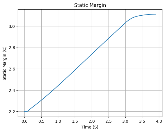
Danger
Always check the static margin of your rocket.
If it is negative, your rocket is unstable and the simulation will most likely fail.
If it is unreasonably high, your rocket is super stable and the simulation will most likely fail.
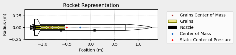
To guarantee that the rocket is stable, the positions of all added components
must be correct. The Rocket class can help you with the draw method:
calisto.draw()
Running the Simulation#
To simulate a flight, we need to create a Flight object.
This object will run the simulation and store the results.
To do this, we need to specify the environment in which the rocket will fly and the rocket itself. We must also specify the length of the launch rail, the inclination of the launch rail and the heading of the launch rail.
test_flight = Flight(
    rocket=calisto, environment=env, rail_length=5.2, inclination=85, heading=0
    )
All simulation information will be saved in the test_flight object.
RocketPy has two submodules to access the results of the simulation: prints
and plots. Each class has its prints and plots submodule imported as
an attribute. For example, to access the prints submodule of the Flight
object, we can use test_flight.prints.
Also, each class has its own methods to quickly access all the information, for
example, the test_flight.all_info() for visualizing all the plots and
the test_flight.info() for a summary of the numerical results.
Bellow we describe how to access and manipulate the results of the simulation.
Accessing numerical results#
Note
All the methods that are used in this section can be accessed at once by
running test_flight.info().
You may want to start by checking the initial conditions of the simulation. This will allow you to check the state of the rocket at the time of ignition:
test_flight.prints.initial_conditions()
Initial Conditions

Initial time: 0.000 s
Position - x: 0.00 m | y: 0.00 m | z: 1471.47 m
Velocity - Vx: 0.00 m/s | Vy: 0.00 m/s | Vz: 0.00 m/s
Attitude (quaternions) - e0: 0.923 | e1: -0.040 | e2: 0.017 | e3: 0.382
Euler Angles - Spin φ : 45.00° | Nutation θ: -5.00° | Precession ψ: 0.00°
Angular Velocity - ω1: 0.00 rad/s | ω2: 0.00 rad/s | ω3: 0.00 rad/s
Initial Stability Margin: 2.199 c
Also important to check the surface wind conditions at launch site and the conditions of the launch rail:
test_flight.prints.surface_wind_conditions()
Surface Wind Conditions

Frontal Surface Wind Speed: -0.05 m/s
Lateral Surface Wind Speed: 0.42 m/s
test_flight.prints.launch_rail_conditions()
Launch Rail

Launch Rail Length: 5.2 m
Launch Rail Inclination: 85.00°
Launch Rail Heading: 0.00°
Once we have checked the initial conditions, we can check the conditions at the out of rail state, which is the first important moment of the flight. After this point, the rocket will start to fly freely:
test_flight.prints.out_of_rail_conditions()
Rail Departure State

Rail Departure Time: 0.368 s
Rail Departure Velocity: 26.208 m/s
Rail Departure Stability Margin: 2.276 c
Rail Departure Angle of Attack: 0.928°
Rail Departure Thrust-Weight Ratio: 10.152
Rail Departure Reynolds Number: 1.828e+05
Next, we can check at the burn out time, which is the moment when the motor stops burning. From this point on, the rocket will fly without any thrust:
test_flight.prints.burn_out_conditions()
Burn out State

Burn out time: 3.900 s
Altitude at burn out: 2130.276 m (ASL) | 658.810 m (AGL)
Rocket speed at burn out: 281.214 m/s
Freestream velocity at burn out: 281.171 m/s
Mach Number at burn out: 0.821
Kinetic energy at burn out: 6.422e+05 J
We can also check the apogee conditions, which is the moment when the rocket reaches its maximum altitude. The apogee will be displayed in both “Above Sea Level (ASL)” and “Above Ground Level (AGL)” formats.
test_flight.prints.apogee_conditions()
Apogee State

Apogee Time: 26.147 s
Apogee Altitude: 4837.618 m (ASL) | 3366.152 m (AGL)
Apogee Freestream Speed: 26.006 m/s
Apogee X position: 9.489 m
Apogee Y position: 584.392 m
Apogee latitude: 32.9955089°
Apogee longitude: -106.9748963°
To check for the ejection of any parachutes, we can use the following method:
test_flight.prints.events_registered()
Parachute Events

Parachute: Drogue
	Ejection time: 26.152 s
	Inflation time: 27.652 s
	Freestream speed at inflation: 29.763 m/s
	Altitude at inflation: 4826.685 m (ASL) | 3355.219 m (AGL)
Parachute: Main
	Ejection time: 158.933 s
	Inflation time: 160.433 s
	Freestream speed at inflation: 18.426 m/s
	Altitude at inflation: 2244.476 m (ASL) | 773.010 m (AGL)
To understand the conditions at the end of the simulation, especially upon impact, we can use:
test_flight.prints.impact_conditions()
Impact Conditions

Time of impact: 294.935 s
X impact: -607.718 m
Y impact: 113.808 m
Altitude impact: 1471.466 m (ASL) | -0.000 m (AGL)
Latitude: 32.9912772°
Longitude: -106.9815132°
Vertical velocity at impact: -5.624 m/s
Number of parachutes triggered until impact: 2
Finally, the prints.maximum_values() provides a summary of the maximum
values recorded during the flight for various parameters.
test_flight.prints.maximum_values()
Maximum Values

Maximum Speed: 287.013 m/s at 3.39 s
Maximum Mach Number: 0.837 Mach at 3.40 s
Maximum Reynolds Number: 1.934e+06 at 3.34 s
Maximum Dynamic Pressure: 3.958e+04 Pa at 3.36 s
Maximum Acceleration During Motor Burn: 105.255 m/s² at 0.15 s
Maximum Gs During Motor Burn: 10.733 g at 0.15 s
Maximum Acceleration After Motor Burn: 61.841 m/s² at 160.44 s
Maximum Gs After Motor Burn: 6.306 Gs at 160.44 s
Maximum Stability Margin: 3.682 c at 3.90 s
Maximum Upper Rail Button Normal Force: 0.019 N
Maximum Upper Rail Button Shear Force: 0.182 N
Maximum Lower Rail Button Normal Force: 0.035 N
Maximum Lower Rail Button Shear Force: 0.327 N
Plotting the Results#
Note
All the methods that are used in this section can be accessed at once by
running test_flight.all_info(). The output will be equivalent to
running block by block the following methods.
Using the test_flight.plots module, we can access multiple results of the
simulation. For example, we can plot the rocket’s trajectory. Moreover, we can
get plots of multiple data:
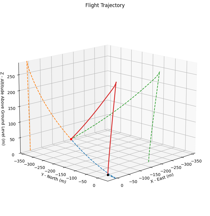
Full trajectory#
test_flight.plots.trajectory_3d()
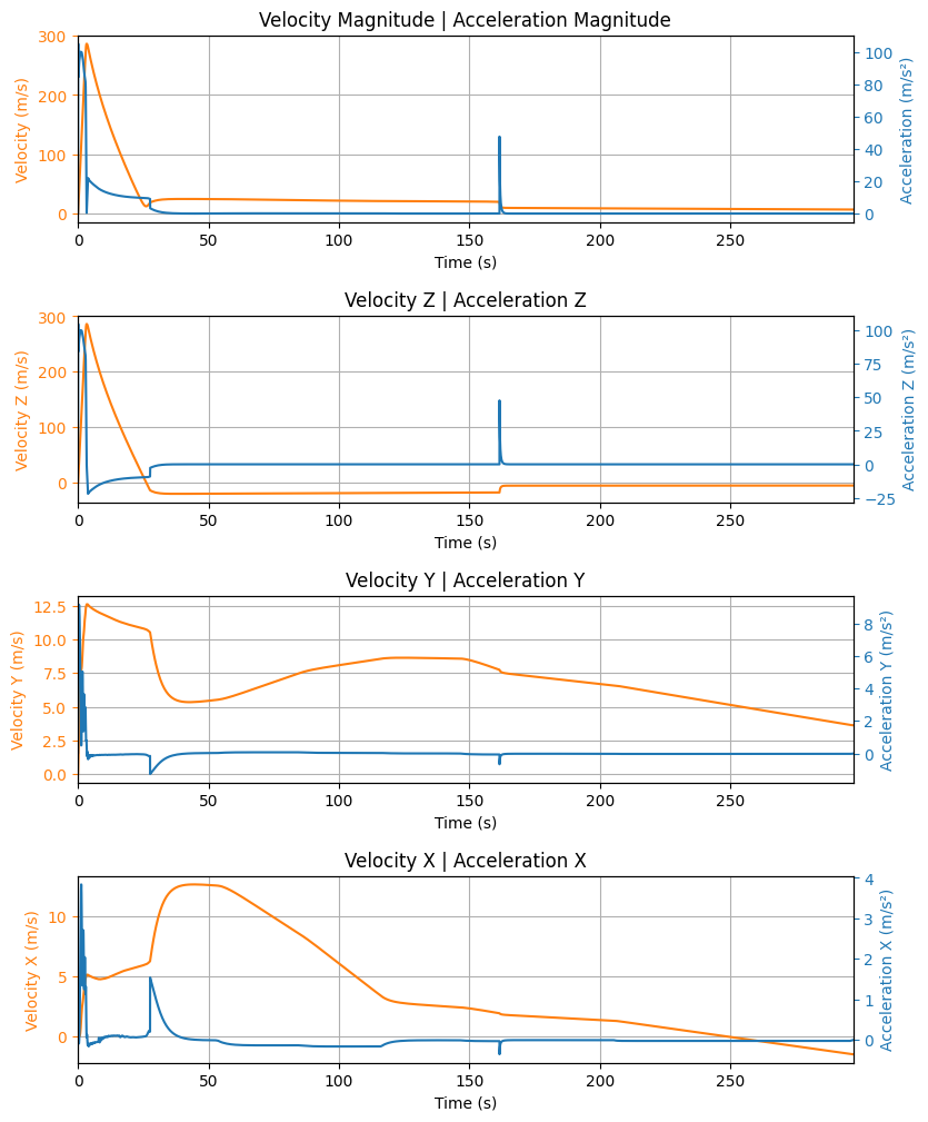
Velocity and acceleration#
The velocity and acceleration in 3 directions can be accessed using the following method. The reference frame used for these plots is the absolute reference frame, which is the reference frame of the launch site. The acceleration might have a hard drop when the motor stops burning.
test_flight.plots.linear_kinematics_data()
Angular Positions#
Here you can plot 3 different parameters of the rocket’s angular position:
Flight Path Angle: The angle between the rocket’s velocity vector and the horizontal plane. This angle is 90° when the rocket is going straight up and 0° when the rocket is turned horizontally.Attitude Angle: The angle between the axis of the rocket and the horizontal plane.Lateral Attitude Angle: The angle between the rockets axis and the vertical plane that contains the launch rail. The bigger this angle, the larger is the deviation from the original heading of the rocket.
test_flight.plots.flight_path_angle_data()
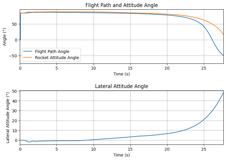
Tip
The Flight Path Angle and the Attitude Angle should be close to each
other as long as the rocket is stable.
Rocket’s Orientation or Attitude#
Rocket’s orientation in RocketPy is done through Euler Parameters or Quaternions. Additionally, RocketPy uses the quaternions to calculate the Euler Angles (Precession, nutation and spin) and their changes. All these information can be accessed through the following method:
test_flight.plots.attitude_data()
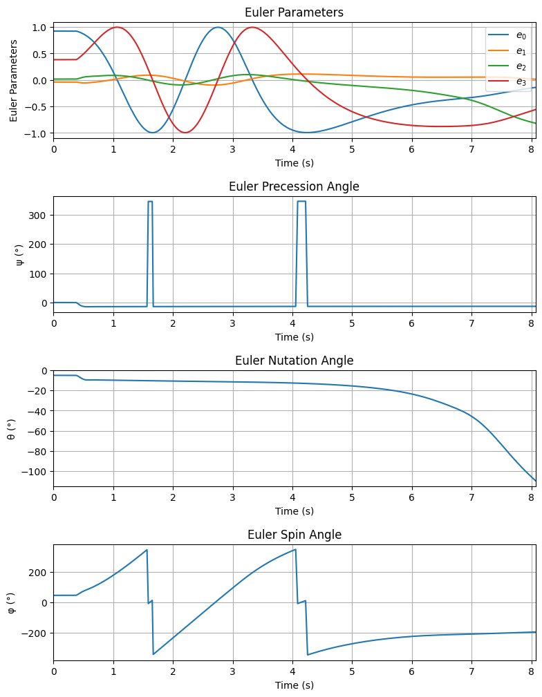
See also
Further information about Euler Parameters, or Quaternions, can be found in Quaternions, while further information about Euler Angles can be found in Euler Angles.
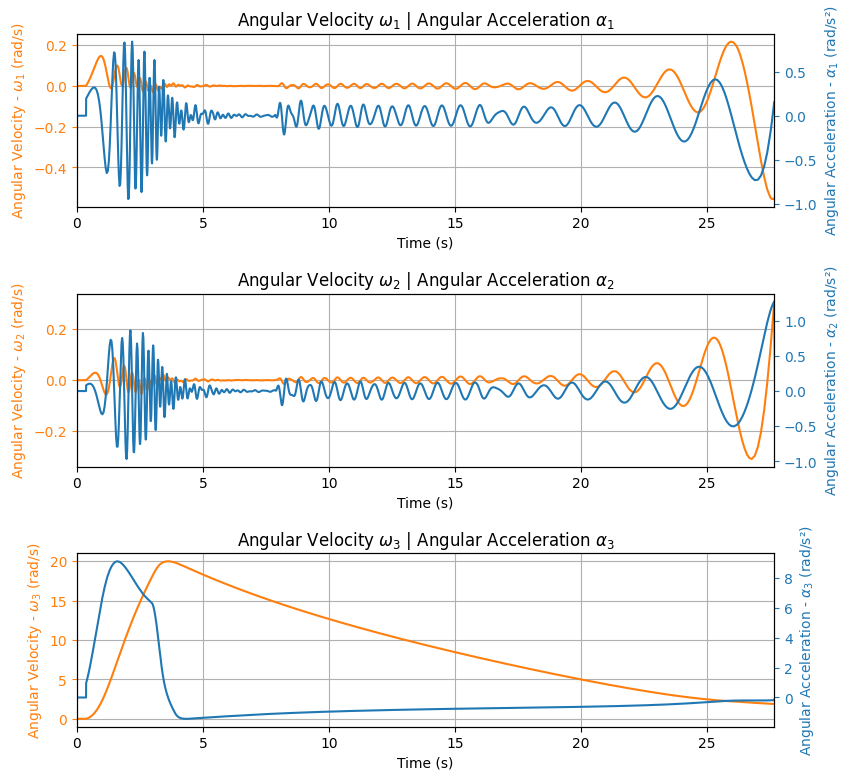
Angular Velocity and Acceleration#
The angular velocity and acceleration are particularly important to check the stability of the rocket. You may expect a sudden change in the angular velocity and acceleration when the motor stops burning, for example:
test_flight.plots.angular_kinematics_data()
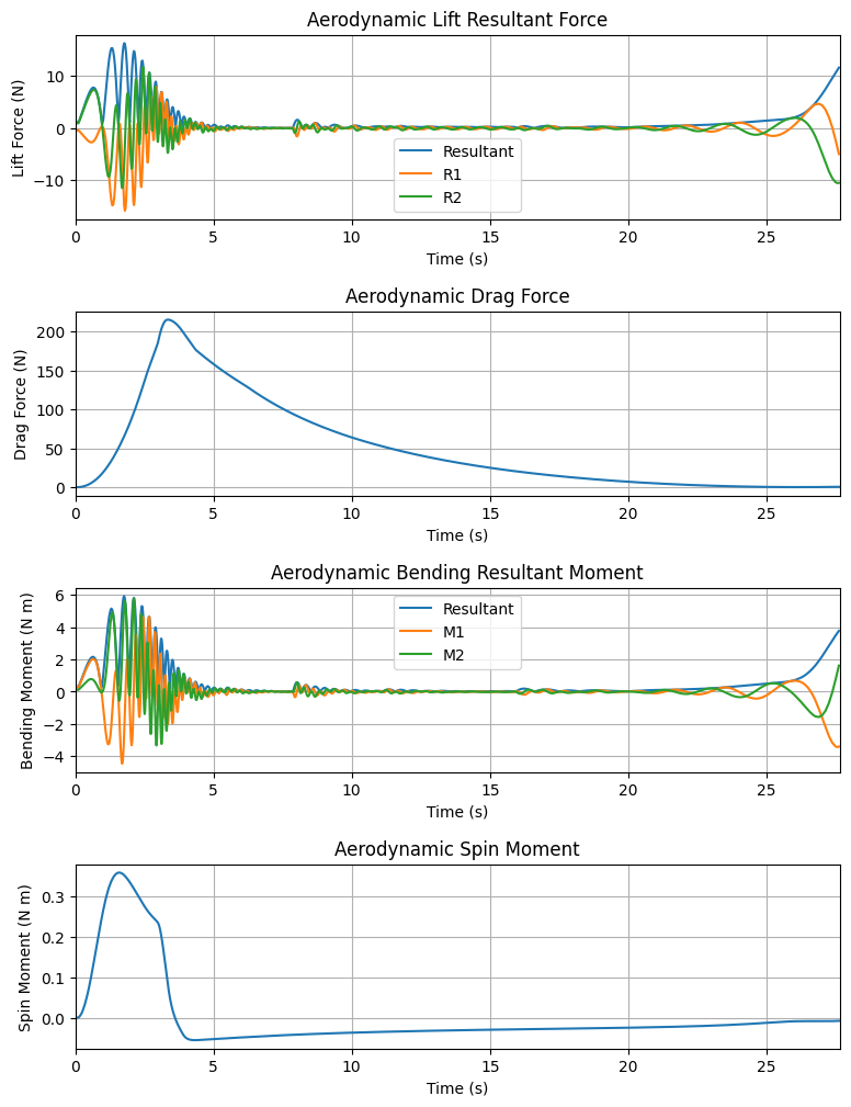
Aerodynamic forces and moments#
The aerodynamic forces and moments are also important to check the flight behavior of the rocket. The drag (axial) and lift forces are made available, as well as the bending and spin moments. The lift is decomposed in two directions orthogonal to the drag force.
test_flight.plots.aerodynamic_forces()
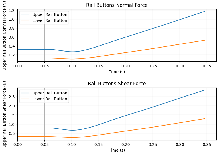
Forces Applied to the Rail Buttons#
RocketPy can also plot the forces applied to the rail buttons before the rocket leaves the rail. This information may be useful when designing the rail buttons and the launch rail.
test_flight.plots.rail_buttons_forces()
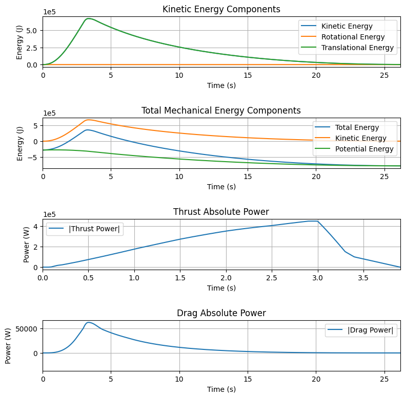
Energies and Power#
RocketPy also calculates the kinetic and potential energy of the rocket during the flight, as well as the thrust and drag power:
test_flight.plots.energy_data()
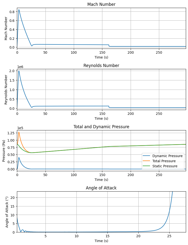
Fluid Mechanics Related Parameters#
RocketPy computes the Mach Number, Reynolds Number, total and dynamic pressure felt by the rocket and the rocket’s angle of attack, all available through the following method:
test_flight.plots.fluid_mechanics_data()
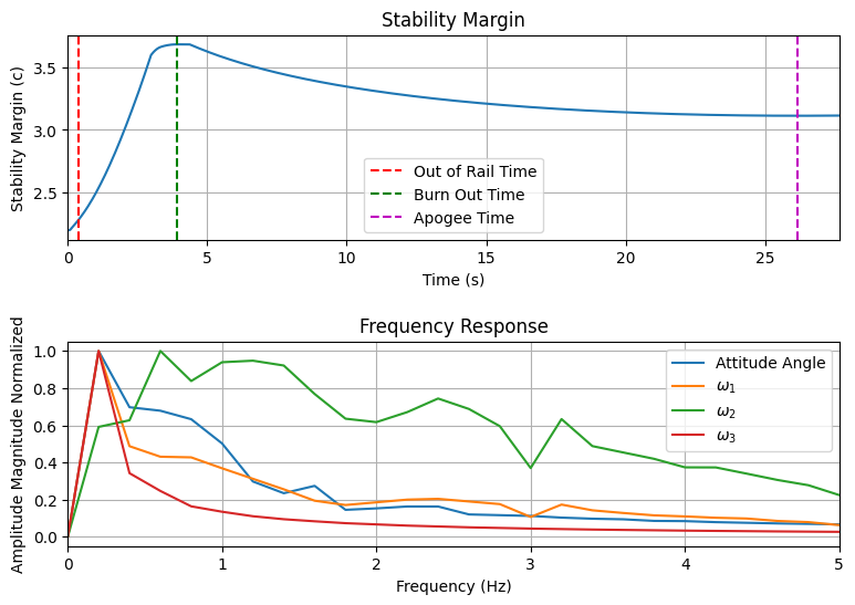
Stability Margin and Frequency Response#
The Stability margin can be checked along with the frequency response of the rocket:
test_flight.plots.stability_and_control_data()
Visualizing the Trajectory in Google Earth#
We can export the trajectory to .kml to visualize it in Google Earth:
Use the dedicated exporter class:
from rocketpy.simulation import FlightDataExporter

FlightDataExporter(test_flight).export_kml(
    file_name="trajectory.kml",
    extrude=True,
    altitude_mode="relativetoground",
)
Note
To learn more about the .kml format, see
KML Reference.
Note
The legacy method Flight.export_kml was removed in v1.13.0. Use
rocketpy.simulation.flight_data_exporter.FlightDataExporter.export_kml().
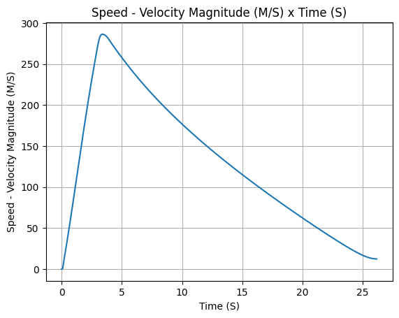
Manipulating results#
There are several methods to access the results. For example, we can plot the speed of the rocket until the first parachute is deployed:
test_flight.speed.plot(0, test_flight.apogee_time)
Or get the array of the speed of the entire flight, in the form
of [[time, speed], ...]:
test_flight.speed.source
array([[0.00000000e+00, 0.00000000e+00],
       [1.40954286e-03, 0.00000000e+00],
       [2.81908573e-03, 0.00000000e+00],
       ...,
       [2.91459617e+02, 5.64459315e+00],
       [2.94209865e+02, 5.64100261e+00],
       [2.94935048e+02, 5.64005935e+00]], shape=(1356, 2))
See also
The Flight object has several attributes containing every result of the
simulation. To see all the attributes of the Flight object, see
rocketpy.Flight. These attributes are usually instances of the
rocketpy.Function class, see the Function Class Usage for more information.
Exporting Flight Data#
In this section, we will explore how to export specific data from your RocketPy simulations to CSV files. This is particularly useful if you want to insert the data into spreadsheets or other software for further analysis.
The recommended API is
rocketpy.simulation.flight_data_exporter.FlightDataExporter.export_data(),
which exports selected flight attributes to a CSV file. In this first example,
we export the rocket angle of attack (see rocketpy.Flight.angle_of_attack())
and the rocket Mach number (see rocketpy.Flight.mach_number()) to the file
calisto_flight_data.csv.
from rocketpy.simulation import FlightDataExporter

exporter = FlightDataExporter(test_flight)
exporter.export_data(
    "calisto_flight_data.csv",
    "angle_of_attack",
    "mach_number",
)
pandas.read_csv():import pandas as pd
pd.read_csv("calisto_flight_data.csv")
| # Time (s) | Angle of Attack (°) | Mach Number | |
|---|---|---|---|
| 0 | 0.000000 | 89.470697 | 0.001234 |
| 1 | 0.001410 | 89.470697 | 0.001234 |
| 2 | 0.002819 | 89.470697 | 0.001234 |
| 3 | 0.005638 | 89.470697 | 0.001234 |
| 4 | 0.008457 | 89.470697 | 0.001234 |
| ... | ... | ... | ... |
| 1351 | 287.561361 | 60.284816 | 0.016323 |
| 1352 | 288.709368 | 60.284509 | 0.016317 |
| 1353 | 291.459617 | 60.284260 | 0.016302 |
| 1354 | 294.209865 | 60.284185 | 0.016288 |
| 1355 | 294.935048 | 60.284177 | 0.016284 |
1356 rows × 3 columns
time_step argument:exporter.export_data(
"calisto_flight_data.csv",
"angle_of_attack",
"mach_number",
time_step=1.0,
)
pd.read_csv("calisto_flight_data.csv")
| # Time (s) | Angle of Attack (°) | Mach Number | |
|---|---|---|---|
| 0 | 0.0 | 89.470697 | 0.001234 |
| 1 | 1.0 | 0.156822 | 0.251636 |
| 2 | 2.0 | 0.034848 | 0.539116 |
| 3 | 3.0 | -0.000000 | 0.795049 |
| 4 | 4.0 | 0.039254 | 0.815177 |
| ... | ... | ... | ... |
| 290 | 290.0 | 60.284328 | 0.016310 |
| 291 | 291.0 | 60.284275 | 0.016305 |
| 292 | 292.0 | 60.284243 | 0.016300 |
| 293 | 293.0 | 60.284212 | 0.016294 |
| 294 | 294.0 | 60.284189 | 0.016289 |
295 rows × 3 columns
This exports the same data at a sampling rate of 1 second. The flight data is interpolated to match the new sampling rate.
Finally, FlightDataExporter.export_data also provides a convenient way to
export the entire flight solution (see rocketpy.Flight.solution_array())
by not passing any attribute names:
exporter.export_data("calisto_flight_data.csv")
Note
The legacy method Flight.export_data was removed in v1.13.0. Use
rocketpy.simulation.flight_data_exporter.FlightDataExporter.export_data().
Saving and Storing Plots#
Here we show how to save the plots and drawings generated by RocketPy.
For instance, we can save our rocket drawing as a .png file:
calisto.draw(filename="calisto_drawing.png")
Also, if you want to save a specific rocketpy plot, every RocketPy
attribute of type rocketpy.Function is capable of saving its plot
as an image file. For example, we can save our rocket’s speed plot and the
trajectory plot as .jpg files:
test_flight.speed.plot(filename="speed_plot.jpg")
test_flight.plots.trajectory_3d(filename="trajectory_plot.jpg")
The supported file formats are .eps, .jpg, .jpeg, .pdf,
.pgf, .png, .ps, .raw, .rgba, .svg, .svgz,
.tif, .tiff and .webp. More details on manipulating data and
results can be found in the Function Class Usage.
Note
The filename argument is optional. If not provided, the plot will be
shown instead. If the provided filename is in a directory that does not
exist, the directory will be created.
Further Analysis#
With the results of the simulation in hand, we can perform a lot of different analysis. Here we will show some examples, but much more can be done!
See also
RocketPy can be used to perform a Monte Carlo Dispersion Analysis. See Monte Carlo Simulations for more information.
Apogee as a Function of Mass#
This one is a classic! We always need to know how much our rocket’s apogee will change when our payload gets heavier.
from rocketpy.utilities import apogee_by_mass

apogee_by_mass(
    flight=test_flight, min_mass=5, max_mass=20, points=10, plot=True
    )

'Function from R1 to R1 : (Rocket Mass without motor (kg)) → (Apogee AGL (m))'
Out of Rail Speed as a Function of Mass#
Lets make a really important plot. Out of rail speed is the speed our rocket has when it is leaving the launch rail. This is crucial to make sure it can fly safely after leaving the rail.
A common rule of thumb is that our rocket’s out of rail speed should be 4 times the wind speed so that it does not stall and become unstable.
from rocketpy.utilities import liftoff_speed_by_mass

liftoff_speed_by_mass(
    flight=test_flight, min_mass=5, max_mass=20, points=10, plot=True
    )

'Function from R1 to R1 : (Rocket Mass without motor (kg)) → (Out of Rail Speed (m/s))'
Dynamic Stability Analysis#
Ever wondered how static stability translates into dynamic stability? Different static margins result in different dynamic behavior, which also depends on the rocket’s rotational inertial.
Let’s make use of RocketPy’s helper class called Function to explore how the dynamic stability of Calisto varies if we change the fins span by a certain factor.
# Helper class
from rocketpy import Function
import copy

# Prepare a copy of the rocket
calisto2 = copy.deepcopy(calisto)

# Prepare Environment Class
custom_env = Environment()
custom_env.set_atmospheric_model(type="custom_atmosphere", wind_v=-5)

# Simulate Different Static Margins by Varying Fin Position
simulation_results = []

for factor in [-0.5, -0.2, 0.1, 0.4, 0.7]:
    # Modify rocket fin set by removing previous one and adding new one
    calisto2.aerodynamic_surfaces.pop(-1)

    fin_set = calisto2.add_trapezoidal_fins(
        n=4,
        root_chord=0.120,
        tip_chord=0.040,
        span=0.100,
        position=-1.04956 * factor,
    )
    # Simulate
    test_flight = Flight(
        rocket=calisto2,
        environment=custom_env,
        rail_length=5.2,
        inclination=90,
        heading=0,
        max_time_step=0.01,
        max_time=5,
        terminate_on_apogee=True,
        verbose=False,
    )
    # Store Results
    static_margin_at_ignition = calisto2.static_margin(0)
    static_margin_at_out_of_rail = calisto2.static_margin(test_flight.out_of_rail_time)
    static_margin_at_steady_state = calisto2.static_margin(test_flight.t_final)
    simulation_results += [
        (
            test_flight.attitude_angle,
            "{:1.2f} c | {:1.2f} c | {:1.2f} c".format(
                static_margin_at_ignition,
                static_margin_at_out_of_rail,
                static_margin_at_steady_state,
            ),
        )
    ]

Function.compare_plots(
    simulation_results,
    lower=0,
    upper=1.5,
    xlabel="Time (s)",
    ylabel="Attitude Angle (deg)",
)
