Function Class Usage#
The rocketpy.Function class in RocketPy is an auxiliary module that allows for easy manipulation of datasets and Python functions. Some of the class features are data interpolation, extrapolation, algebra and plotting.
The basic steps to create a Function are as follows:
Define a data source: a dataset (e.g. x,y coordinates) or a function that maps a dataset to a value (e.g. \(f(x) = x^2\));
Construct a
Functionobject with this dataset assource;Use the
Functionfeatures as needed: add datasets, integrate at a point, make a scatter plot and much more.
These basic steps are detailed in this guide.
1. Define a Data Source#
a. Datasets#
The Function class supports a wide variety of dataset sources:
List or Numpy Array#
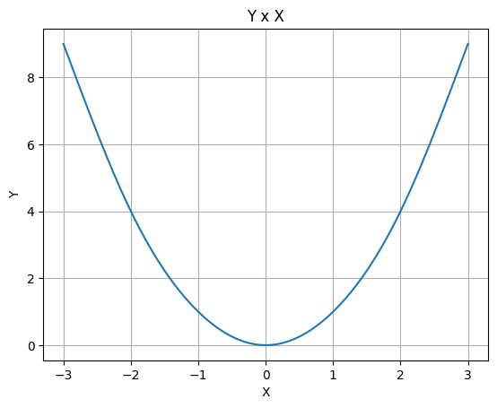
A list or numpy.ndarray of datapoints that maps input values to an output can be used as a Function source. For instance, we can define a dataset that follows the function \(f(x) = x^2\):
from rocketpy.mathutils import Function

# Source dataset [(x0, y0), (x1, y1), ...]
source = [
    (-3, 9), (-2, 4), (-1, 1),
    (0, 0), (1, 1), (2, 4),
    (3, 9)
    ]

# Create a Function object with this dataset
f = Function(source, "x", "y")
One may print the source attribute from the Function object to check the input dataset.
# Print the source to see the dataset
print(f.source)
[[-3.  9.]
 [-2.  4.]
 [-1.  1.]
 [ 0.  0.]
 [ 1.  1.]
 [ 2.  4.]
 [ 3.  9.]]
Furthermore, in order to visualize the dataset, one may use the plot method
from the Function object:
# Plot the source with standard spline interpolation
f.plot()
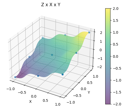
The dataset can be defined as a multidimensional array (more than one input maps to an output), where each row is a data point. For example, let us define a dataset that follows the plane \(z = x + y\):
# Source dataset [(x0, y0, z0), (x1, y1, z1), ...]
source = [
    (-1, -1, -2), (-1, 0, -1), (-1, 1, 0),
    (0, -1, -1), (0, 0, 0), (0, 1, 1),
    (1, -1, 0), (1, 0, 1), (1, 1, 2)
    ]

# Create a Function object with this dataset
f = Function(source, ["x", "y"], "z")
One may print the source attribute from the Function object to check the
input dataset.
print(f.source)
[[-1. -1. -2.]
 [-1.  0. -1.]
 [-1.  1.  0.]
 [ 0. -1. -1.]
 [ 0.  0.  0.]
 [ 0.  1.  1.]
 [ 1. -1.  0.]
 [ 1.  0.  1.]
 [ 1.  1.  2.]]
Two dimensional plots are also supported, therefore this data source can be plotted as follows:
# Plot the source with standard 2d shepard interpolation
f.plot()
Important
For datasets higher than one dimension (more than one input), the
Function class supports interpolation linear, shepard, rbf
and regular_grid.
The regular_grid interpolation requires a complete Cartesian grid and
must be provided as (axes, grid_data). See the Function API
documentation for details.
CSV File#
A CSV file path can be passed as string to the Function source.
The file must contain a dataset structured so that each line is a data point:
the last column is the output and the previous columns are the inputs.
# Create a csv and save with pandas
import pandas as pd

df = pd.DataFrame({
    '"x"': [-3, -2, -1, 0, 1, 2, 3],
    '"y"': [9, 4, 1, 0, 1, 4, 9],
    })
df.to_csv('source.csv', index=False)
pd.read_csv('source.csv')
| "x" | "y" | |
|---|---|---|
| 0 | -3 | 9 |
| 1 | -2 | 4 |
| 2 | -1 | 1 |
| 3 | 0 | 0 |
| 4 | 1 | 1 |
| 5 | 2 | 4 |
| 6 | 3 | 9 |
Having the csv file, we can define a Function object with it:
# Create a Function object with this dataset
f = Function('source.csv')

# One may even delete the csv file
import os
os.remove('source.csv')

# Print the source to see the dataset
print(f.source)
[[-3.  9.]
 [-2.  4.]
 [-1.  1.]
 [ 0.  0.]
 [ 1.  1.]
 [ 2.  4.]
 [ 3.  9.]]
Note
A single header line in the csv file is optional.
b. Function Map#
A Python function that maps a set of parameters to a result can be used as a Function source. For instance, we can define a function that maps x to \(f(x) = \sin(x)\):
import numpy as np
from rocketpy.mathutils import Function

# Define source function
def source_func(x):
    return np.sin(x)

# Create a Function from source
f = Function(source_func)
The result of this operation is a Function object that wraps the source function and features many functionalities, such as plotting.
Constant Functions#
A special case of the python function source is the definition of a constant Function. The class supports a convenient shortcut to ease the definition of a constant source:
# Constant function
f = Function(1.5)

print(f(0))
1.5
Note
This shortcut is completely equivalent to defining a Python constant function as the source:
def const_source(_):
    return 1.5

g = Function(const_source)
2. Building your Function#
In this section we are going to delve deeper on Function creation and its parameters:
source: the
Functiondata source. We have explored this parameter in the section above;inputs: a list of strings containing each input variable name. If the source only has one input, may be abbreviated as a string (e.g. “speed (m/s)”);
outputs: a list of strings containing each output variable name. If the source only has one output, may be abbreviated as a string (e.g. “total energy (J)”);
interpolation: a string that is the interpolation method to be used if the source is a dataset. For N-D datasets, supported options are
linear,shepard,rbfandregular_grid. Defaults tosplinefor 1-D andshepardfor N-D datasets;extrapolation: a string that is the extrapolation method to be used if the source is a dataset. Defaults to
constant;title: the title to be shown in the plots.
See also
Check out more about the constructor parameters and other functionalities in the rocketpy.Function documentation.
With these in mind, let us create a more concrete example so that each of these parameters usefulness is explored.
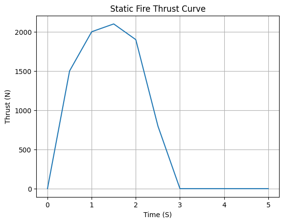
Suppose we have a dataset containing the data from a static fire test of a rocket engine in testing phase. The dataset contain has a column for time (s) and thrust (N). We want to create a Function object that represents the thrust curve of this engine.
from rocketpy.mathutils import Function

# Static fire data
motor_thrust = [
    (0, 0), (0.5, 1500), (1, 2000),
    (1.5, 2100), (2, 1900), (2.5, 800),
    (3, 0)
    ]

# Create a Function object with this dataset
thrust = Function(
    source=motor_thrust,
    inputs="time (s)",
    outputs="thrust (N)",
    interpolation="spline",
    extrapolation="zero",
    title="Static Fire Thrust Curve"
    )
The parameters interpolation and extrapolation are of particular importance in this example:
Due the fact the data is quite sparse, we want to use a
splineinterpolation to smooth the curve.The extrapolation method is set to
zerobecause we know that the thrust is zero before and after the test.
Let’s plot this curve to visualize the effect of these options in action:
# Plotting from 0 to 5 seconds
thrust.plot(0, 5)

Now lets visualize what happens if we were to use a linear interpolation and a constant extrapolation:
# Change interpolation and extrapolation
thrust.set_interpolation("linear")
thrust.set_extrapolation("constant")

# Plotting from 0 to 5 seconds
thrust.plot(0, 5)
3. Function Features#
The Function class has many features that can be used to manipulate the source data. In this section we are going to explore some of these features, such as Function call, Function arithmetic, discretization, differentiation and integration.
a. Function Call#
A Function objects maps input data to an output, therefore should you want to get an output value from a given input, this can be accomplished by the method rocketpy.Function.get_value():
from rocketpy.mathutils import Function

f = Function(lambda x: x**0.5)

print(f.get_value(9))
3.0
Equivalently, the same operation is defined by the Python dunder method
__call__ so that the object can be used like a common function.
For instance:
print(f(9), f(25))
3.0 5.0
Note
A dunder method is a method that is surrounded by double underscores, such as __call__. These methods are used by Python to implement operator overloading.
Furthermore, both the rocketpy.Function.get_value() and the dunder
__call__ method can be used to get a list of outputs from a list of inputs:
# Using __call__
print(f([1, 4, 9, 16, 25]))

# Using get_value
print(f.get_value([1, 4, 9, 16, 25]))
[1.0, 2.0, 3.0, 4.0, 5.0]
[1.0, 2.0, 3.0, 4.0, 5.0]
b. Function Arithmetic#
An important feature of the Function class is the ability to perform
arithmetic operations between real values or even other Function objects.
The following operations are supported:
Addition:
+;Subtraction:
-;Multiplication:
*;Division:
/;Exponentiation:
**.
Let’s see some examples of these operations:
import numpy as np

f = Function(lambda x: np.sin(x))

g = f/4 + 1

Function.compare_plots([f, g], lower=0, upper=4*np.pi)

Note
This is an example of the static method rocketpy.Function.compare_plots(), it is used to plot Functions in the same graph for comparison.
Arithmetic can also be performed on sets of data of the same length and same domain discretization (i.e. equal x values):
source1 = [(0, 0), (0.5, 0.25), (1, 1), (1.5, 2.25), (2, 4)]
source2 = [(0, 0), (0.5, 0.5), (1, 1), (1.5, 1.5), (2, 2)]

f = Function(source1)
g = Function(source2)

h = (f + g) / 2

Function.compare_plots([f, g, h], lower=0, upper=2)

c. Discretization#
The Function class can also convert from function sourced to a discretized dataset produced from it. This is accomplished by the method rocketpy.Function.set_discrete() and allows for a great computational speed up if the function source is complex.
The accuracy of the discretization depends on the number of datapoints and the chosen interpolation method.
Let’s compare the discretization of a sine function:
import numpy as np
from copy import copy

# Function from sine
f = Function(lambda x: np.sin(x))

# Discretization
f_continuous = copy(f)
f_discrete = f.set_discrete(
    lower=0,
    upper=4*np.pi,
    samples=20,
    interpolation="linear"
    )

Function.compare_plots([f_continuous, f_discrete], lower=0, upper=4*np.pi)

Important
A copy of the original continuous function was necessary in this example, since the method rocketpy.Function.set_discrete() mutates the original Function.
d. Differentiation and Integration#
One of the most useful Function features for data analysis is easily differentiating and integrating the data source. These methods are divided as follow:
rocketpy.Function.differentiate(): differentiate theFunctionat a given point, returning the derivative value as the result;rocketpy.Function.differentiate_complex_step(): differentiate theFunctionat a given point using the complex step method, returning the derivative value as the result;rocketpy.Function.integral(): performs a definite integral over specified limits, returns the integral value (area underFunction);rocketpy.Function.derivative_function(): computes the derivative of the given Function, returning another Function that is the derivative of the original at each point;rocketpy.Function.integral_function(): calculates the definite integral of the function from a given point up to a variable, returns aFunction.
Derivatives#
Let’s make a familiar example of differentiation: the derivative of the function \(f(x) = x^2\) is \(f'(x) = 2x\). We can use the Function class to compute those:
# Define the function x^2
f = Function(lambda x: x**2)

# Differentiate it at x = 3
print(f.differentiate(3))
6.000000000838668
RocketPy also supports the complex step method for differentiation, which is a very accurate method for numerical differentiation. Let’s compare the results of the complex step method with the standard method:
# Define the function x^2
f = Function(lambda x: x**2)

# Differentiate it at x = 3 using the complex step method
print(f.differentiate_complex_step(3))
6.0
The complex step method can be as twice as faster as the standard method, but it requires the function to be differentiable in the complex plane.
Also one may compute the derivative function:
# Define the function x^2 and its derivative
f = Function(lambda x: x**2)
f_dot = f.derivative_function()

# Compare their plots
Function.compare_plots([f, f_dot], lower=-2, upper=2)

Integrals#
Now, to illustrate the power of the Function class in making it easy to make plots of complex functions, let’s plot the integral of the gaussian function:
Which is non-elementary so it cannot be expressed in terms of common functions.
# Define the gaussian function
def gaussian(x):
    return 1 / np.sqrt(2*np.pi) * np.exp(-x**2/2)

f = Function(gaussian)

# Integrate from 0 to 1
print(f.integral(0,1))
0.341344746068543
Here we have shown that we can integrate the gaussian function over a defined interval, let’s compute its integral function.
# Compute the integral function from -4
f_int = f.integral_function(-4, 4, 1000)

# Compare the function with the integral
Function.compare_plots([f, f_int], lower=-4, upper=4)

e. Export to a text file (CSV or TXT)#
Since rocketpy version 1.2.0, the Function class supports exporting the
source data to a CSV or TXT file. This is accomplished by the method
rocketpy.Function.savetxt() and allows for easy data exportation for
further analysis.
Let’s export the gaussian function to a CSV file:
# Define the gaussian function
def gaussian(x):
    return 1 / np.sqrt(2*np.pi) * np.exp(-x**2/2)

f = Function(gaussian, inputs="x", outputs="f(x)")

# Export to CSV
f.savetxt("gaussian.csv", lower=-4, upper=4, samples=20, fmt="%.2f")

# Read the CSV file
import pandas as pd
pd.read_csv("gaussian.csv")
| x | f(x) | |
|---|---|---|
| 0 | -4.00 | 0.00 |
| 1 | -3.58 | 0.00 |
| 2 | -3.16 | 0.00 |
| 3 | -2.74 | 0.01 |
| 4 | -2.32 | 0.03 |
| 5 | -1.89 | 0.07 |
| 6 | -1.47 | 0.13 |
| 7 | -1.05 | 0.23 |
| 8 | -0.63 | 0.33 |
| 9 | -0.21 | 0.39 |
| 10 | 0.21 | 0.39 |
| 11 | 0.63 | 0.33 |
| 12 | 1.05 | 0.23 |
| 13 | 1.47 | 0.13 |
| 14 | 1.89 | 0.07 |
| 15 | 2.32 | 0.03 |
| 16 | 2.74 | 0.01 |
| 17 | 3.16 | 0.00 |
| 18 | 3.58 | 0.00 |
| 19 | 4.00 | 0.00 |
# Delete the CSV file
import os
os.remove("gaussian.csv")
f. Filter data#
Since rocketpy version 1.2.0, the Function class supports filtering the
source data. This is accomplished by the method rocketpy.Function.low_pass_filter()
and allows for easy data filtering for further analysis.
Let’s filter an example function:
x = np.linspace(-4, 4, 1000)
y = np.sin(x) + np.random.normal(0, 0.1, 1000)

f = Function(list(zip(x, y)), inputs="x", outputs="f(x)")

# Filter the function
f_filtered = f.low_pass_filter(0.5)

# Compare the function with the filtered function
Function.compare_plots(
    [(f, "Original"), (f_filtered, "Filtered")], lower=-4, upper=4
)

This guide shows some of the capabilities of the Function class, but there are many other functionalities to enhance your analysis. Do not hesitate in tanking a look at the documentation rocketpy.Function.