Air Brakes#
Air brakes are commonly used in rocketry to slow down a rocket’s ascent. They are usually deployed to make sure that the rocket reaches a certain altitude.
Lets make a simple air brakes example. We will use the same model as in the First Simulation example, but we will add a simple air brakes model.
Setting Up The Simulation#
First, lets define everything we need for the simulation up to the rocket:
from rocketpy import Environment, SolidMotor, Rocket, Flight

env = Environment(latitude=32.990254, longitude=-106.974998, elevation=1400)

Pro75M1670 = SolidMotor(
    thrust_source="../data/motors/cesaroni/Cesaroni_M1670.eng",
    dry_mass=1.815,
    dry_inertia=(0.125, 0.125, 0.002),
    nozzle_radius=33 / 1000,
    grain_number=5,
    grain_density=1815,
    grain_outer_radius=33 / 1000,
    grain_initial_inner_radius=15 / 1000,
    grain_initial_height=120 / 1000,
    grain_separation=5 / 1000,
    grains_center_of_mass_position=0.397,
    center_of_dry_mass_position=0.317,
    nozzle_position=0,
    burn_time=3.9,
    throat_radius=11 / 1000,
    coordinate_system_orientation="nozzle_to_combustion_chamber",
)

calisto = Rocket(
    radius=127 / 2000,
    mass=14.426,
    inertia=(6.321, 6.321, 0.034),
    power_off_drag="../data/rockets/calisto/powerOffDragCurve.csv",
    power_on_drag="../data/rockets/calisto/powerOnDragCurve.csv",
    center_of_mass_without_motor=0,
    coordinate_system_orientation="tail_to_nose",
)

rail_buttons = calisto.set_rail_buttons(
    upper_button_position=0.0818,
    lower_button_position=-0.618,
    angular_position=45,
)

calisto.add_motor(Pro75M1670, position=-1.255)

nose_cone = calisto.add_nose(
    length=0.55829, kind="vonKarman", position=1.278
)

fin_set = calisto.add_trapezoidal_fins(
    n=4,
    root_chord=0.120,
    tip_chord=0.060,
    span=0.110,
    position=-1.04956,
    cant_angle=0.5,
    airfoil=("../data/airfoils/NACA0012-radians.txt","radians"),
)

tail = calisto.add_tail(
    top_radius=0.0635, bottom_radius=0.0435, length=0.060, position=-1.194656
)
Setting Up the Air Brakes#
Now we can get started!
To create an air brakes model, we essentially need to define the following:
The air brakes’ drag coefficient as a function of the air brakes’ deployment level and of the Mach number. This can be done through a
CSVfile which must have three columns: the first column is the air brakes’ deployment level, the second column is the Mach number, and the third column is the drag coefficient added to rocket due to the air brakes at that specific deployment level and Mach number.The controller function, which takes in as argument information about the simulation up to the current time step, and the
AirBrakesinstance being defined, and sets the desired air brakes’ deployment level. The air brakes’ deployment level must be between 0 and 1, and is set using thedeployment_levelattribute. Inside this function, any controller logic, filters, and apogee prediction can be implemented.The sampling rate of the controller function, in seconds. This is the time between each call of the controller function, in simulation time. Must be given in Hertz.
Defining the Controller Function#
Lets start by defining a very simple controller function.
The controller_function must take in the following arguments, in this
order:
time(float): The current simulation time in seconds.sampling_rate(float): The rate at which the controller function is called, measured in Hertz (Hz).state(list): The state vector of the simulation. The state is a list containing the following values, in this order:x: The x position of the rocket, in meters.y: The y position of the rocket, in meters.z: The z position of the rocket, in meters.v_x: The x component of the velocity of the rocket, in meters per second.v_y: The y component of the velocity of the rocket, in meters per second.v_z: The z component of the velocity of the rocket, in meters per second.e0: The first component of the quaternion representing the rotation of the rocket.e1: The second component of the quaternion representing the rotation of the rocket.e2: The third component of the quaternion representing the rotation of the rocket.e3: The fourth component of the quaternion representing the rotation of the rocket.w_x: The x component of the angular velocity of the rocket, in radians per second.w_y: The y component of the angular velocity of the rocket, in radians per second.w_z: The z component of the angular velocity of the rocket, in radians per second.
state_history(list): A record of the rocket’s state at each step throughout the simulation. The state_history is organized as a list of lists, with each sublist containing a state vector. The last item in the list always corresponds to the previous state vector, providing a chronological sequence of the rocket’s evolving states.observed_variables(list): A list containing the variables that the controller function returns. The return of each controller function call is appended to the observed_variables list. The initial value in the first step of the simulation of this list is provided by theinitial_observed_variablesargument.air_brakes(AirBrakes): TheAirBrakesinstance being controlled.
Our example controller_function will deploy the air brakes when the rocket
reaches 1500 meters above the ground. The deployment level will be function of the
vertical velocity at the current time step and of the vertical velocity at the
previous time step.
Also, the controller function will check for the burnout of the rocket’s motor and only deploy the air brakes if the rocket has reached burnout.
Then, a limitation for the opening/closing speed of the air brakes will be set. The air brakes deployment level will not be able to change faster than 20% per second, in our case.
Lets define the controller function:
def controller_function(
    time, sampling_rate, state, state_history, observed_variables, air_brakes, sensors, environment
):
    # state = [x, y, z, vx, vy, vz, e0, e1, e2, e3, wx, wy, wz]
    altitude_ASL = state[2]
    altitude_AGL = altitude_ASL - environment.elevation
    vx, vy, vz = state[3], state[4], state[5]

    # Get winds in x and y directions
    wind_x, wind_y = environment.wind_velocity_x(altitude_ASL), environment.wind_velocity_y(altitude_ASL)

    # Calculate Mach number
    free_stream_speed = (
        (wind_x - vx) ** 2 + (wind_y - vy) ** 2 + (vz) ** 2
    ) ** 0.5
    mach_number = free_stream_speed / environment.speed_of_sound(altitude_ASL)

    # Get previous state from state_history
    previous_state = state_history[-1]
    previous_vz = previous_state[5]

    # If we wanted to we could get the returned values from observed_variables:
    # returned_time, deployment_level, drag_coefficient = observed_variables[-1]

    # Check if the rocket has reached burnout
    if time < Pro75M1670.burn_out_time:
        return None

    # If below 1500 meters above ground level, air_brakes are not deployed
    if altitude_AGL < 1500:
        air_brakes.deployment_level = 0

    # Else calculate the deployment level
    else:
        # Controller logic
        new_deployment_level = (
            air_brakes.deployment_level + 0.1 * vz + 0.01 * previous_vz**2
        )

        # Limiting the speed of the air_brakes to 0.2 per second
        # Since this function is called every 1/sampling_rate seconds
        # the max change in deployment level per call is 0.2/sampling_rate
        max_change = 0.2 / sampling_rate
        lower_bound = air_brakes.deployment_level - max_change
        upper_bound = air_brakes.deployment_level + max_change
        new_deployment_level = min(max(new_deployment_level, lower_bound), upper_bound)

        air_brakes.deployment_level = new_deployment_level

    # Return variables of interest to be saved in the observed_variables list
    return (
        time,
        air_brakes.deployment_level,
        air_brakes.drag_coefficient(air_brakes.deployment_level, mach_number),
    )
Note
The
controller_functionaccepts 6, 7, or 8 parameters for backward compatibility:6 parameters (original):
time,sampling_rate,state,state_history,observed_variables,air_brakes7 parameters (with sensors): adds
sensorsas the 7th parameter8 parameters (with environment): adds
sensorsandenvironmentas the 7th and 8th parameters
The environment parameter provides access to atmospheric conditions (wind, temperature, pressure, elevation) without relying on global variables. This enables proper serialization of rockets with air brakes and improves code modularity. Available methods include
environment.elevation,environment.wind_velocity_x(altitude),environment.wind_velocity_y(altitude),environment.speed_of_sound(altitude), and others.The code inside the
controller_functioncan be as complex as needed. Anything can be implemented inside the function, including filters, apogee prediction, and any controller logic.The
air_brakesinstancedeployment_levelis clamped between 0 and 1. This means that the deployment level will never be set to a value lower than 0 or higher than 1. If you want to disable this feature, setclamptoFalsewhen defining the air brakes.Anything can be returned by the
controller_function. The returned values will be saved in theobserved_variableslist at every time step and can then be accessed by thecontroller_functionat the next time step. The saved values can also be accessed after the simulation is finished. This is useful for debugging and for plotting the results.The
controller_functioncan also be defined in a separate file and imported into the simulation script. This includes importing acorcppcode into Python.
Defining the Drag Coefficient#
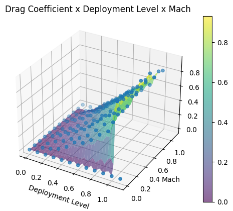
Now lets define the drag coefficient as a function of the air brakes’ deployment level and of the Mach number. We will import the data from a CSV file.
The CSV file must have three columns: the first column must be the air brakes’ deployment level, the second column must be the Mach number, and the third column must be the drag coefficient.
Alternatively, the drag coefficient can be defined as a function of the air brakes’ deployment level and of the Mach number. This function must take in the air brakes’ deployment level and the Mach number as arguments, and must return the drag coefficient.
Note
At deployment level 0, the drag coefficient will always be set to 0, regardless of the input curve. This means that the simulation considers that at a deployment level of 0, the air brakes are completely retracted and do not contribute to the drag of the rocket.
Part of the data from the CSV can be seen in the code block below.
deployment_level, mach, cd
0.0, 0.0, 0.0
0.1, 0.0, 0.0
0.1, 0.2, 0.0
0.1, 0.3, 0.01
0.1, 0.4, 0.005
0.1, 0.5, 0.006
0.1, 0.6, 0.018
0.1, 0.7, 0.012
0.1, 0.8, 0.014
0.5, 0.1, 0.051
0.5, 0.2, 0.051
0.5, 0.3, 0.065
0.5, 0.4, 0.061
0.5, 0.5, 0.067
0.5, 0.6, 0.083
0.5, 0.7, 0.08
0.5, 0.8, 0.085
1.0, 0.1, 0.32
1.0, 0.2, 0.225
1.0, 0.3, 0.225
1.0, 0.4, 0.21
1.0, 0.5, 0.19
1.0, 0.6, 0.22
1.0, 0.7, 0.21
1.0, 0.8, 0.218
Note
The air brakes’ drag coefficient curve can represent either the air brakes
alone or both the air brakes and the rocket. This is determined by the
override_rocket_drag argument. If set to True, the drag
coefficient curve will include both the air brakes and the rocket. If set to
False, the curve will exclusively represent the air brakes.
When the curve represents only the air brakes, its drag coefficient will be added to the rocket’s existing drag coefficient. Conversely, if the curve represents both the air brakes and the rocket, the drag coefficient will be set to match that of the curve. This feature is particularly useful when you have a drag coefficient curve for the entire rocket with the air brakes deployed, such as data from a wind tunnel test, and you want to incorporate it into the simulation.
Adding the Air Brakes to the Rocket#
Now we can add the air brakes to the rocket.
We will set the reference_area to None. This means that the reference
area for the calculation of the drag force from the coefficient will be the
rocket’s reference area (the area of the cross section of the rocket). If we
wanted to set a different reference area, we would set reference_area to
the desired value.
Also, we will set clamp to True. This means that the deployment level will
be clamped between 0 and 1. This means that the deployment level will never be set
to a value lower than 0 or higher than 1. This can alter the behavior of the
controller function. If you want to disable this feature, set clamp to
False.
air_brakes = calisto.add_air_brakes(
    drag_coefficient_curve="../data/rockets/calisto/air_brakes_cd.csv",
    controller_function=controller_function,
    sampling_rate=10,
    reference_area=None,
    clamp=True,
    initial_observed_variables=[0, 0, 0],
    override_rocket_drag=False,
    name="Air Brakes",
)

air_brakes.all_info()
Note
The initial_observed_variables argument is optional. It is used as
the initial value for the observed_variables list passed on the
controller_function at the first time step. If not given, the
observed_variables list will be initialized as an empty list.
See also
For more information on the rocketpy.AirBrakes class
initialization, see rocketpy.AirBrakes.__init__ section.
Simulating a Flight#
Important
To simulate the air brakes successfully, we must set time_overshoot to
False. This way the simulation will run at the time step defined by our
controller sampling rate. Be aware that this will make the simulation run
much slower.
We will be terminating the simulation at apogee, by setting
terminate_at_apogee to True. This way the simulation will stop when the
rocket reaches apogee, and we will save some time.
test_flight = Flight(
    rocket=calisto,
    environment=env,
    rail_length=5.2,
    inclination=85,
    heading=0,
    time_overshoot=False,
    terminate_on_apogee=True,
)
Analyzing the Results#
Now we can create some plots to analyze the results. We rely on the
observed_variables list to get the data we want to plot. Since we returned
the time, deployment_level and the drag_coefficient in the
controller_function, the observed_variables list will contain these
values at every time step.
We can retrieve the observed_variables list by calling the
get_controller_observed_variables method of the Flight instance.
Then we can plot the data we want.
import matplotlib.pyplot as plt
time_list, deployment_level_list, drag_coefficient_list = [], [], []
obs_vars = test_flight.get_controller_observed_variables()
for time, deployment_level, drag_coefficient in obs_vars:
time_list.append(time)
deployment_level_list.append(deployment_level)
drag_coefficient_list.append(drag_coefficient)
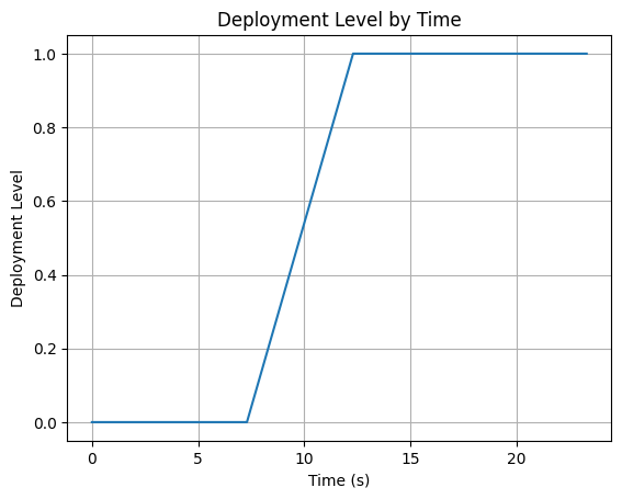
# Plot deployment level by time
plt.plot(time_list, deployment_level_list)
plt.xlabel("Time (s)")
plt.ylabel("Deployment Level")
plt.title("Deployment Level by Time")
plt.grid()
plt.show()
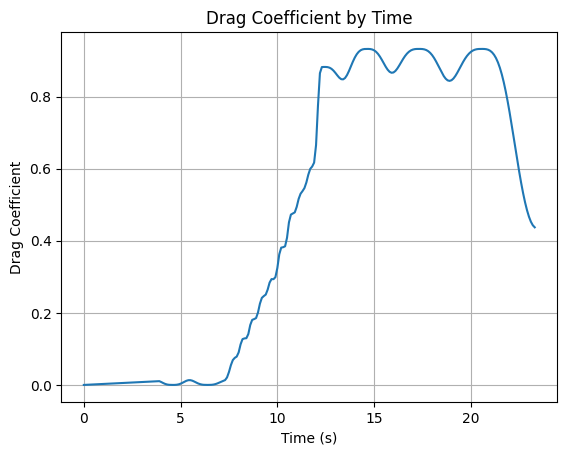
# Plot drag coefficient by time
plt.plot(time_list, drag_coefficient_list)
plt.xlabel("Time (s)")
plt.ylabel("Drag Coefficient")
plt.title("Drag Coefficient by Time")
plt.grid()
plt.show()
See also
For more information on the rocketpy.AirBrakes class attributes,
see rocketpy.AirBrakes section.
And of course, we should check some of the simulation results:
test_flight.prints.burn_out_conditions()
test_flight.prints.apogee_conditions()
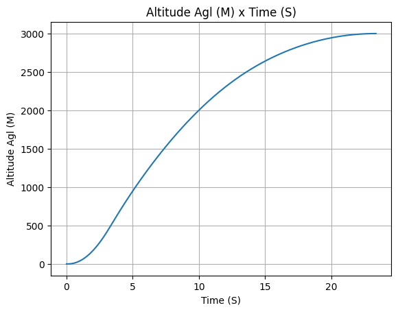
test_flight.altitude()
test_flight.vz()
Burn out State

Burn out time: 3.900 s
Altitude at burn out: 2057.373 m (ASL) | 657.373 m (AGL)
Rocket speed at burn out: 279.644 m/s
Freestream velocity at burn out: 279.644 m/s
Mach Number at burn out: 0.843
Kinetic energy at burn out: 6.350e+05 J

Apogee State

Apogee Time: 22.776 s
Apogee Altitude: 4302.839 m (ASL) | 2902.839 m (AGL)
Apogee Freestream Speed: 15.591 m/s
Apogee X position: -3.800 m
Apogee Y position: 465.700 m
Apogee latitude: 32.9944416°
Apogee longitude: -106.9750387°